The maximum norm is the largest absolute vector component. Use it for symmetric position caps and worst-error tolerances, with clear units and limits on its risk interpretation.
Maximum norm
The maximum norm, also called the infinity norm, measures a vector by its largest absolute component. For a vector of holdings it answers “how big is the biggest position?” For a vector of model errors it answers “how bad is the worst individual error?”
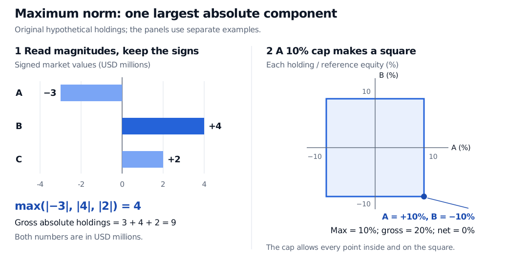
Suppose a hypothetical desk holds three cash-equity positions with signed market values, in USD millions,
x=(−3,4,2).
The short position has magnitude 3, and the two longs have magnitudes 4 and 2. Therefore
∥x∥∞=4,∥x∥1=9,∥x∥2=29≈5.385165.
All three results carry the same USD-million unit, but answer different questions. The Manhattan norm adds the absolute holdings, giving gross market value. The Euclidean norm combines their squares. Neither Euclidean length nor maximum position size is automatically portfolio volatility.
For an actual limit, define each signed weight wi as the position's market value divided by the same positive reference equity. A symmetric 10% limit is
∥w∥∞≤0.10⟺−0.10≤wi≤0.10for every i.
The limit treats longs and shorts symmetrically. It supplies neither a budget constraint nor a long-only condition. In two dimensions the allowed region is a square; in three it is a cube. In general it is a box aligned with the chosen coordinates, a convex set.
Original hypothetical examples. Holdings minus 3, plus 4 and plus 2 USD millions have maximum norm 4 and gross absolute value 9. A separate two-holding square permits each signed weight between minus 10% and plus 10%; its plus 10%, minus 10% corner has maximum norm 10%, gross exposure 20% and net exposure zero.
Original hypothetical holdings. The left panel uses USD millions; the separate right panel uses percentages of a common reference equity. The square includes its boundary.
A cap on each holding is not a cap of the same size on total exposure. The two-holding book (0.10,−0.10) passes the limit, yet has 20% gross exposure and zero net exposure. For n holdings, the cap only implies ∥w∥1≤0.10n. Portfolio risk still depends on the assets, their dependence, liquidity and the relevant payoff model. For derivatives, a cap on market value alone may say little about underlying exposure.
For the square example, dividing each weight by its explicit 0.10 cap gives dimensionless coordinates (1,−1). Their maximum norm is 1: the book sits on the boundary. Its Manhattan norm is 2 and Euclidean norm is 2. These scaled coordinates refer to this two-holding illustration, not the three-position USD vector above.
Worst error, common scale
For two equal-length vectors, the corresponding distance is
d∞(x,y)=∥x−y∥∞=imax∣xi−yi∣.
If three model-minus-observed quote errors are (0.03,−0.01,0.02)USD per share, their maximum norm is USD 0.03 per share. Requiring this norm to be at most a tolerance means every quote must pass. It does not let many accurate quotes compensate for one large error.
That interpretation requires comparable coordinates. Taking a maximum across raw dollar errors, volatility errors and basis-point errors is unit-dependent. With explicit positive tolerances si, use
imaxsi∣xi−yi∣≤1.
This is a dimensionless maximum of tolerance utilisation. Changing the tolerances changes what counts as a large error; the scaling is part of the model.
Why it behaves like a length
The maximum norm is zero only at the zero vector, and scaling gives ∥ax∥∞=∣a∣∥x∥∞. Its triangle inequality follows coordinate by coordinate:
∣xi+yi∣≤∣xi∣+∣yi∣≤∥x∥∞+∥y∥∞.
Taking the maximum over i proves the result. It also compares with Euclidean length through
∥x∥∞≤∥x∥2≤n∥x∥∞.
The largest squared component is at most the sum of squares; each of the n squared components is at most the largest squared component. That proves both bounds and explains why the dimension enters the upper one.
Check the object as well as the subscript. The induced infinity matrix norm is the largest absolute row sum, not the largest individual entry. The vector definition above should not be applied to a matrix without stating the intended convention.
For the underlying holdings arithmetic, Vectors and Matrices develops ordered components, portfolio weights and factor exposures. For constraints inside an optimiser, Constrained and Convex Optimisation explains feasible sets and inequality constraints. Both full lessons require membership, with public previews.
Sources
Lloyd N. Trefethen and David Bau III, Numerical Linear Algebra, SIAM, 1997, Lecture 3, pp. 17–19, equations (3.1)–(3.4): norm properties, vector p-norms, unit balls and weighted norms; p. 21, Example 3.4 and equation (3.10), for the induced infinity matrix norm.