Survey ratio and regression estimator: Definition & Examples

Survey ratio and regression estimators use a known population total or mean of an auxiliary variable to adjust an estimate of another population quantity. A quant auditing fees, positions or operational records can use a complete, inexpensive size measure to improve an estimate based on a smaller, expensive reconciliation sample. The target is a population total or mean, rather than an individual prediction or a causal regression coefficient.

Suppose the population contains

N

accounts. For account

i

x_i

is a recorded transaction count and

y_i

is a fee amount established by an audit. The total transaction count

X=\sum_{i=1}^N x_i

is known; the fee total

Y=\sum_{i=1}^N y_i

is not. The formulas below assume simple random sampling of

n

accounts without replacement, with both variables observed on each selected account. Write

\bar X=X/N

for the population auxiliary mean and

\bar x,\bar y

for sample means.

Two ways to correct the same imbalance

The plain expansion estimate is $\widehat Y_0=N\bar y$ . It ignores any mismatch between the sample's transaction count and the population's known count.

The ratio estimator uses the observed fee-per-transaction ratio:

r=\frac{\bar y}{\bar x}=\frac{\sum_{i\in s}y_i}{\sum_{i\in s}x_i}, \qquad \widehat Y_R=rX,

where

s

denotes the selected accounts and

\bar x\ne0

. It is attractive when fees are approximately proportional to transaction counts, with a relationship near the origin. A small or unstable denominator makes the ratio unreliable. Columbia's survey-sampling notes, lecture 6, develop this auxiliary-total construction.

The regression estimator permits an intercept. Fit ordinary least squares to the sampled pairs:

b=\frac{\sum_{i\in s}(x_i-\bar x)(y_i-\bar y)}{\sum_{i\in s}(x_i-\bar x)^2}, \qquad a=\bar y-b\bar x.

Then use the known auxiliary mean:

\widehat Y_{\mathrm{reg}} =N\left[\bar y+b(\bar X-\bar x)\right] =Na+bX.

The denominator defining

b

must be positive. The fitted slope converts the auxiliary imbalance into a correction to the total. Penn State's regression-estimation notes explain this population estimator and its approximate sampling uncertainty.

The two corrections can be written together:

\widehat Y_R=N\bar y+r(X-N\bar x), \qquad \widehat Y_{\mathrm{reg}}=N\bar y+b(X-N\bar x).

They use different slopes to adjust the same discrepancy. If $\bar x=\bar X$ , both return the plain expansion estimate.

A four-account audit

In this fictional example, $N=100$ accounts have a known total of $X=1{,}200$ transactions for one day. Four accounts selected by simple random sampling are audited:

Account	Transactions $x_i$	Daily fees $y_i$ (USD)
A	8	16
B	10	19
C	12	25
D	10	20
Sample total	40	80

Thus $\bar x=10$ , $\bar y=20$ USD and $\bar X=12$ . The sample has fewer transactions per account than the population. The three estimates are:

Estimator	Calculation	Estimated population fees (USD)
Plain expansion	$100\times20$	2,000
Ratio	$1{,}200\times(80/40)$	2,400
Regression	$100\left[20+2.25(12-10)\right]$	2,450

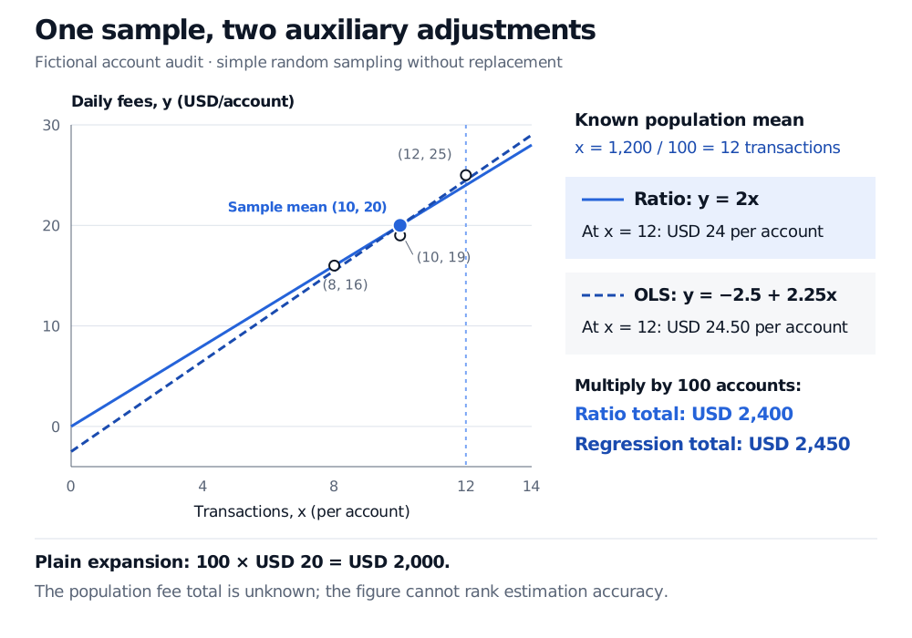
For the regression, the centred cross-product sum is $18$ and the centred sum of squared transaction counts is $8$ , giving $b=18/8=2.25$ and $a=-2.5$ . The ratio is $r=2$ . At the known population mean of 12 transactions, the ratio line gives USD 24 per account and the regression line gives USD 24.50.

Fictional four-account audit: ratio line y equals 2x and OLS line y equals minus 2.5 plus 2.25x both pass through the sample mean of 10 transactions and USD 20. At the known population mean of 12 transactions they imply USD 24 and USD 24.50 per account, or totals USD 2,400 and USD 2,450.

The auxiliary adjustment changes the estimate from the sample's account mix to the known population transaction count. The actual population fee total is not supplied, so none of these numbers establishes which estimate is closer to the truth.

The negative fitted intercept is an extrapolation of this small sample's line. It does not establish that a zero-transaction account earns a negative fee.

A ratio line is not automatically a no-intercept OLS fit

Although

y=rx

passes through the origin, its slope

\sum y_i/\sum x_i

generally differs from the unweighted no-intercept OLS slope

\sum x_i y_i/\sum x_i^2

. Choosing “omit intercept” in a regression routine therefore need not reproduce the survey ratio estimate. Victoria University's survey notes, §12.4, distinguish the ratio construction from the constant-error-variance no-intercept model.

For the intercept fit used here, Least Squares and Regression Geometry explains the fitted line and residual orthogonality. Its preview is public; full teaching requires membership.

Precision depends on the sampling design

Under repeated simple random samples, $N\bar y$ is design-unbiased. The ratio and sample-fitted regression estimators are generally not exactly design-unbiased: both reuse random sample quantities in their adjustments. Large-sample bias and variance approximations require regularity, including a stable auxiliary denominator for the ratio.

Precision gains depend on residual variation around the chosen relationship. Strong correlation alone does not make the origin restriction appropriate. Regression variance is commonly approximated using the fitted residual mean square, scaled by $N^2(1-n/N)/n$ . Here $1-n/N$ is the finite-population correction; the residual mean square uses divisor $n-2$ for an intercept and one slope. With only four sampled accounts, the calculation above illustrates the estimators rather than supporting a dependable large-sample confidence interval.

The known total must describe the same units, eligibility rules and period as the target. If it is itself estimated, its uncertainty must enter the analysis. Unequal inclusion probabilities, stratification, clustering and nonresponse require appropriate survey weights and design-specific variance calculations. Treating survey weights as ordinary precision weights can change the estimand or uncertainty calculation; auxiliary adjustment does not automatically repair missing coverage or selective response.

Sources

Columbia University, Survey Sampling (Fall 2006), lectures 6–7, PDF pages 13–17: ratio and regression population estimation, residual-based variance, and the distinction between fixed and estimated adjustment slopes.
Penn State, STAT 506, Lesson 4: Auxiliary Data and Ratio Estimation, §4.1–4.2: known auxiliary totals, proportional relationships and ratio-estimator bias.
Penn State, STAT 506, Lesson 5: Auxillary Data and Regression Estimation, §5.1–5.2: regression mean/total estimators, approximate variance and comparisons with expansion and ratio estimation.
Richard Arnold, Victoria University of Wellington, STAT392: Sample Surveys, Chapter 12, §12.1 and §12.4: sampling weights, auxiliary-based totals and the ratio-model distinction.

Two ways to correct the same imbalance

A four-account audit

A ratio line is not automatically a no-intercept OLS fit

Precision depends on the sampling design

Sources

Related terms

Cluster sampling

Ordinary least squares

Population

Simple random sampling

Stratified sampling