A shadow rate model is a short-rate model in which a latent rate can keep moving below a floor while the model’s nominal short rate stays at that floor. When the overnight market barely moves, changes elsewhere on the yield curve can still help estimate the latent rate and the distribution of future rates.
What the floor hides
Write for the shadow rate, for the model short rate and for the floor. The model applies the floor at every date.
Above the floor, the shadow rate and the model short rate coincide. At the floor, every shadow value at or below gives the same short rate. A single overnight reading near the floor therefore carries little information about how far below it the shadow rate lies. The positive-part term in the formula has the shape of a call option payoff. Black motivated the zero-floor case with the option to hold currency at zero nominal interest. Black, Interest Rates as Options
The floor is an assumption about the particular rate and market being modelled. An effective lower bound can be below zero because storing and handling large amounts of cash costs money. For example, the ECB introduced a negative deposit facility rate of −0.10% in June 2014. BIS analysis of the lower bound · ECB decision
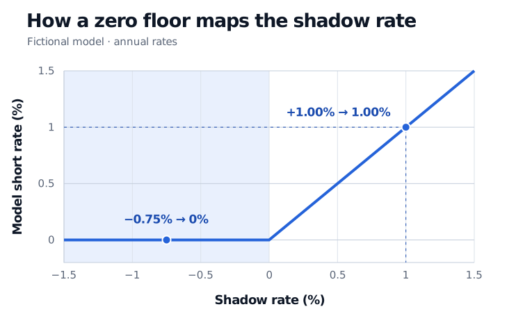
The horizontal segment shows why different shadow rates can produce the same model short rate. Above the kink, the two rates move one for one.
Apply the floor before averaging
In the fictional zero-floor model above, suppose next year’s shadow rate has two equally likely outcomes under the risk-neutral measure. The −0.75% shadow rate maps to 0%, and the +1.00% shadow rate maps to 1.00%. With annual rates throughout, the average after flooring is 0.50%. The average shadow rate is 0.125%, which is already positive, so flooring that average leaves it at 0.125%.
This order matters because the maximum is a convex function. For an integrable future shadow rate , Jensen’s inequality gives
The inequality is strict when there is positive probability on both sides of the floor. The downside scenarios stop at the floor while the upside scenarios retain their full effect.
Price the rate path before quoting a forward
The expected floored rate averages possible rates at one date. A zero-coupon bond instead prices the whole short-rate path. In continuous time, the price of one unit paid at is the risk-neutral average of the discount factors formed from those paths.
Continue the two-scenario example. The first year’s short rate is known to be 0%, and at the start of the second year the model selects a short rate of 0% or 1.00%, each with risk-neutral probability one half, and holds it for that year. The one-year bond price is 1. The two-year bond price is the average of and . The continuously compounded one-year forward rate for the second year is
The difference from 0.50% comes from averaging the discount factors before taking the logarithm. Wu and Xia use an analytical forward-rate approximation that also accounts for the variability of the cumulative rate path. Wu and Xia, Appendix A
The SelfMadeQuant lesson on the fundamental pricing equation derives path discounting and works through a two-state bond price. The preview is public and the full lesson is for members.
Reading the Wu–Xia series
Wu and Xia estimate the shadow rate from one-month Treasury forward rates at several horizons, using a model with three latent factors and a 0.25% floor in their benchmark specification. A decline in their estimate while the short rate is pinned can summarise easing reflected in the curve, including changes around asset-purchase announcements or forward guidance. The estimated level depends on the floor and the fitted dynamics. It can also reflect moves in the term premium. Wu and Xia, §§2 and 5–6
As of 8 November 2026, the Atlanta Fed still listed its Wu–Xia Shadow Federal Funds Rate updates as suspended. Its 8 April 2022 notice says updates are suspended while the federal funds target range remains above 0–0.25%. The Federal Open Market Committee’s 28 October 2026 statement maintained the range at 3.75–4.00%. Atlanta Fed series notice · October 2026 FOMC statement
Sources
- Fischer Black, Interest Rates as Options, Journal of Finance, 1995. Original zero-floor and option analogy.
- Jing Cynthia Wu and Fan Dora Xia, Measuring the Macroeconomic Impact of Monetary Policy at the Zero Lower Bound, 2015 conference version, §§2 and 5–6 and Appendix A. Model specification, estimation, interpretation and the forward-rate approximation.
- BIS, How have central banks implemented negative policy rates?, March 2016. Discussion of cash-handling costs and the effective lower bound.
- ECB, ECB introduces a negative deposit facility interest rate, 5 June 2014. Announcement and effective date.
- Federal Reserve Bank of Atlanta, Wu-Xia Shadow Federal Funds Rate. Model inputs and the 8 April 2022 suspension notice.
- Federal Reserve Board, FOMC statement of 28 October 2026. Federal funds target range used to check the suspension condition.