Generate a target density with accept–reject sampling: a global envelope, an exact triangular example, acceptance probability and the cost of discarded proposals.
Rejection sampling
Rejection sampling generates a draw from a target distribution by proposing a value from an easier distribution, then accepting it with a carefully chosen probability. Rejected candidates are discarded and the procedure starts again. It is also called the accept–reject algorithm.
In a Monte Carlo simulation, the target might be a modelled loss severity or a bounded risk factor whose density is easy to evaluate but awkward to invert. Rejection sampling supplies the random inputs; it does not establish that the chosen distribution describes market losses.
The envelope does the work
Let f be the target probability density function, and let q be a proposal density that we can sample. Choose a finite constant M satisfying
f(x)≤Mq(x)
throughout the target support. The proposal must cover every region to which the target assigns positive probability. With both densities normalized, necessarily M≥1.
For each attempt:
Draw a candidate X∼q and an independent U∼Uniform(0,1).
Accept X if U≤f(X)/(Mq(X)).
Otherwise discard the pair and retry with fresh independent inputs.
The continuous uniform distribution converts the density ratio into an acceptance probability. Draw candidates from q, not from the scaled curve Mq: the latter integrates to M and generally is not a density.
A tilted distribution from flat proposals
Consider a synthetic, dimensionless risk factor with
f(x)=2x,0≤x≤1,
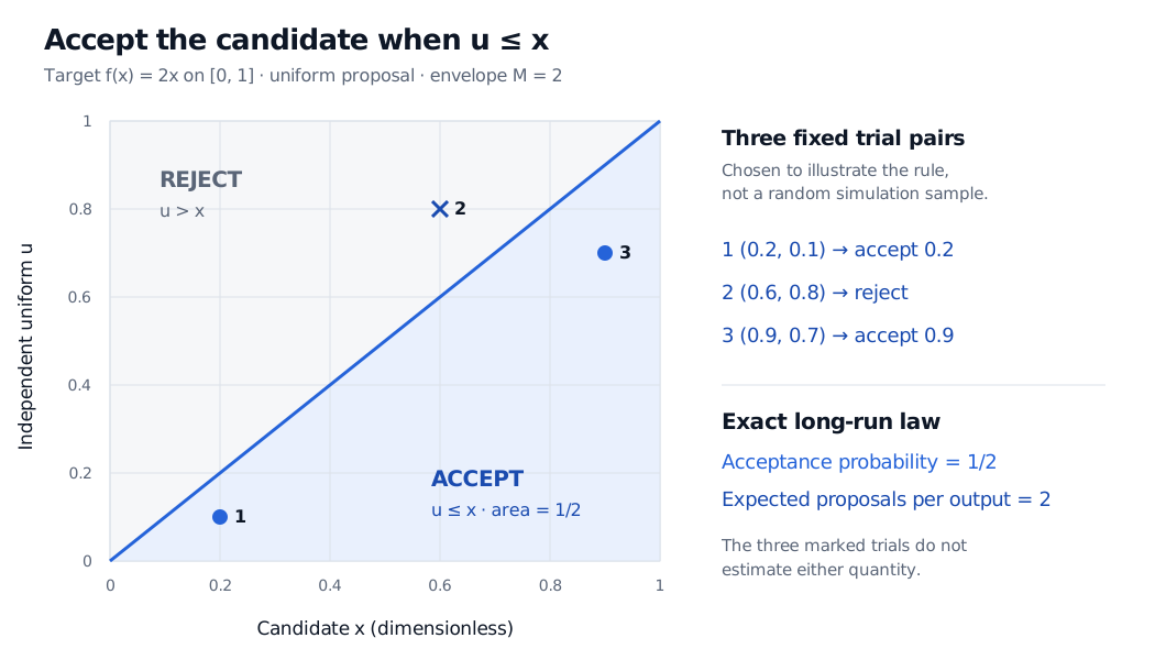
and zero density elsewhere. Its density increases toward one. Use a uniform proposal on [0,1], so q(x)=1 there. The envelope M=2 dominates the entire density, giving
Mq(x)f(x)=x.
Thus a candidate near one is more likely to survive than a candidate near zero. The proposal stays uniform; the acceptance filter changes the distribution of retained values.
Fixed candidate x
Fixed uniform input u
Decision
0.2
0.1
Accept 0.2
0.6
0.8
Reject
0.9
0.7
Accept 0.9
These are deliberately chosen pairs, not random samples. Their two acceptances out of three are not an estimate of the algorithm's acceptance probability.
Unit-square accept–reject construction: accept u at or below x. The triangle has area one half. Fixed pairs (0.2,0.1) and (0.9,0.7) are accepted; (0.6,0.8) is rejected. Exact acceptance probability is one half and expected proposals per output is two.
Original deterministic illustration for the synthetic density f(x)=2x. The marked pairs demonstrate decisions; the area calculation establishes the probability.
The geometry also verifies the output distribution. For 0≤b≤1, the area of the accepted triangle to the left of b is b2/2. Dividing by the whole accepted area, 1/2, gives
P(X≤b∣accepted)=b2.
Its derivative is 2b, exactly the target density. For example, only one quarter of the accepted distribution lies at or below 0.5, although half of the original uniform proposal distribution does.
Why rejection does not bias the target
For any measurable region A, the joint probability of proposing a value in A and accepting is
Over the full support this gives P(accepted)=1/M. Conditioning on acceptance cancels that factor and leaves the target probability ∫Af(x)dx. With independent attempts, the number of proposals up to and including the next acceptance has a geometric distribution, with mean M. Fresh independent inputs also give independent retained draws.
For our example, acceptance probability is 1/2 and the expected cost is two proposals per accepted output. This is an average, not a promise that every second proposal succeeds. The count includes the successful proposal.
A valid bound is more valuable than a convincing plot
An envelope must dominate everywhere relevant, including the tails. A few plotted points or a large observed acceptance rate cannot certify the bound. Missing proposal support loses target outcomes altogether. Using a bound that is too small, then capping the acceptance ratio at one, generally samples the wrong distribution.
A larger valid bound preserves correctness but wastes attempts. In the same example, choosing M=4 reduces acceptance to 1/4 and raises the expected number of proposals to four. Choosing a proposal closer to the target can improve efficiency, provided the global bound remains valid. Cost per proposal matters too: a tighter envelope may require more expensive calculations.
The method can also use an unnormalized target h, provided 0<Z=∫h(x)dx<∞ and a known bound h(x)≤Cq(x) is available. Accept with probability h(X)/(Cq(X)). The output density is h/Z, and acceptance probability is Z/C, not generally 1/C. The unknown normalizing constant cancels from the decision. Luke Tierney's simulation notes develop this envelope formulation and its numerical considerations.
Inverse transform sampling offers a different route when an accurate quantile function is available. For the finance setting and the geometric basis of acceptance–rejection, see Random Number Generation (public preview; full lesson requires membership).
Sources
Geoffrey R. Grimmett and David R. Stirzaker, Probability and Random Processes, third edition (Oxford University Press, 2001), §4.11, Example 5, pp. 123–124: the rejection method and its conditional-distribution argument.