Generate a target distribution from uniform inputs using a generalized inverse CDF, with exact discrete thresholds, an exponential example and explicit endpoint conventions.
Inverse transform sampling
Inverse transform sampling generates a random variable with a chosen distribution by applying its quantile function to a uniform random input. In a risk simulation, it is the step that turns a probability between zero and one into a modelled loss or waiting time. The probabilities come from the stipulated model; the transformation does not estimate them from market data.
If U∼Uniform(0,1), then Q(U) has CDF F. An ordinary inverse is unnecessary: F may have jumps or flat stretches, and no probability density function is required. The rule is to find the first threshold whose cumulative probability reaches the input. University of Ulm, Inversion Method.
A probability interval buys an outcome
Consider this synthetic one-period loss model, in USD:
Loss
Probability
Cumulative probability
USD 0
0.2
0.2
USD 10
0.5
0.7
USD 30
0.3
1
The inverse partitions the unit interval:
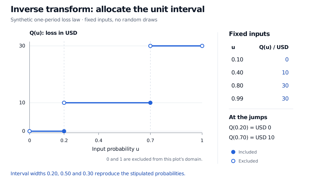
Q(u)=⎩⎨⎧0,10,30,0<u≤0.2,0.2<u≤0.7,0.7<u<1.
Thus the fixed inputs 0.1,0.4,0.8,0.99 give losses 0,10,30,30. These four chosen numbers demonstrate the mapping; they are not random draws or an empirical frequency check.
Generalized inverse loss map: probability intervals of widths 0.2, 0.5 and 0.3 select USD 0, USD 10 and USD 30. Filled endpoints give Q(0.2)=0 and Q(0.7)=10.
Original deterministic illustration of a synthetic one-period loss law. Filled points are included; hollow points are excluded. Fixed probability inputs illustrate the map and are not random simulation draws.
For an ideal uniform input, interval lengths give probabilities: the USD 10 interval has length 0.7−0.2=0.5, exactly its assigned mass. At the jumps, our stated convention gives Q(0.2)=0 and Q(0.7)=10. Interpolating between USD 10 and USD 30 would manufacture losses absent from this model.
Why the whole distribution is correct
For every real x and 0<u<1, the generalized inverse satisfies Q(u)≤x exactly when u≤F(x). Therefore
P(Q(U)≤x)=P(U≤F(x))=F(x).
This establishes the target law at every threshold, not just its mean. Applying Q separately to independent uniform inputs also preserves independence. Reusing one input across different variables can create dependence: correct marginal distributions alone do not define a joint risk model. University of Ulm, Theorem 3.4.
Continuous inversion
Suppose a waiting time T, measured in years, follows an exponential distribution with a stipulated constant rate λ=2 per year. For t≥0,
FT(t)=1−e−2t,QT(u)=−2log(1−u).
Choosing u=1−e−2≈0.864665 gives QT(u)=1 year. Here the inverse solves FT(t)=u exactly. The same law is a Gamma distribution with shape 1 and scale 0.5 year; the scale is the reciprocal rate.
The endpoints belong to the implementation contract
The theorem above uses 0<U<1. An ideal continuous uniform variable hits either endpoint with probability zero. A computer generator uses a finite grid: for example, NumPy's Generator.random returns values in [0,1), which includes zero. That endpoint cannot simply be dismissed as impossible. NumPy documentation.
A generic implementation can require an open-interval uniform source or redraw excluded endpoints. A distribution-specific implementation may instead document endpoint extensions. For this exponential formula, extending to u=0 gives zero waiting time; u=1 gives an infinite wait. Those are different from blindly applying the infimum definition at zero: because every CDF satisfies F(x)≥0, that infimum over all real x is −∞. For the finite loss law, the extension at u=1 is USD 30. There is no universal finite endpoint answer.
For small positive u, evaluate the exponential formula as -log1p(-u)/2 to avoid losing precision in 1−u (NumPy, log1p). More generally, closed-form inverses are often unavailable; numerical inversion needs accuracy checks, especially in the tails. Rejection and other methods may be more efficient for a particular distribution. SciPy's sampling guide.
Sources
Geoffrey R. Grimmett and David R. Stirzaker, Probability and Random Processes, third edition (Oxford University Press, 2001), §4.11, pp. 122–123: inverse-transform sampling, discrete thresholds and exponential constructions.