QLIKE scores variance forecasts against noisy variance proxies. Compare score conventions, asymmetric forecast penalties and the conditional-unbiasedness requirement.
QLIKE loss
QLIKE loss is a quasi-likelihood-based score for comparing positive variance forecasts with observed variance proxies. Lower average loss means a better volatility forecast under this scoring rule. Its practical appeal is that an appropriate noisy proxy can preserve an expected forecast comparison even when the variance being forecast is unobservable.
Score the variance, not its square root
For a positive variance proxy y and positive forecast variance h, a normalised convention is
L(y,h)=hy−log(hy)−1.
The score is nonnegative and zero at h=y. Both inputs must describe the same return, horizon and variance units. A 2% standard deviation becomes 0.022=0.0004 in decimal-return variance; inserting 0.02 directly would score a different object. Variance and volatility are different inputs.
Consider one fictional daily proxy y=0.0004:
Forecast
Daily variance h
Corresponding standard deviation
Normalised QLIKE
A
0.0001
1%
1.6137
B
0.0004
2%
0
C
0.0016
4%
0.6363
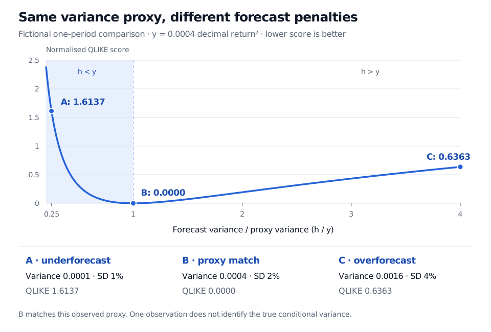
For A, y/h=4, giving 4−log(4)−1≈1.6137. C overshoots variance by a factor of four, whereas A undershoots by that factor; these reciprocal errors receive different penalties. B matches this proxy exactly. That does not establish that B equals the unobserved conditional variance.
Fictional daily variance proxy 0.0004. Forecast A has variance 0.0001 and QLIKE 1.6137; B has variance 0.0004 and score 0; C has variance 0.0016 and score 0.6363. The curve plots normalised QLIKE against forecast variance divided by proxy variance.
Original fictional one-period comparison. The curve holds the proxy fixed; reciprocal fourfold variance errors incur different scores. Standard deviations are shown only as translations of the variance inputs.
Why two QLIKE implementations can report different numbers
The subtracted term is identical across forecasts for the same observation. The conventions therefore rank forecasts identically on the same dates with the same weights, but their reported loss levels differ. The unnormalised score can be negative; zero is not its universal benchmark.
If y=0, the normalised expression is undefined. The unnormalised score remains finite for h>0, with ℓ(0,h)=log(h). Document that convention and investigate whether zeros are valid measurements. An arbitrary positive replacement changes the data. A zero or negative forecast variance is outside either scoring convention's domain.
What proxy robustness actually buys
Let F be the information available when both forecasts are issued. Suppose the nonnegative proxy Y satisfies E[Y∣F]=v, where v>0 is the target conditional variance. Both forecasts must be positive and measurable with respect to F, and the score differences below must be integrable.
That is the difference obtained by inserting v itself. Conditional unbiasedness does the work; unconditional unbiasedness alone is insufficient when forecasts vary with available information. Expected loss levels additionally require the relevant losses to be finite. Patton's §3 sets out the broader regularity conditions for robust loss functions.
For an original two-outcome illustration, keep v=0.0004 and forecasts A and B above. Let the proxy equal 0.0001 or 0.0007, each with conditional probability one-half. Its conditional mean is v. The normalised loss difference, A minus B, is −0.6363 in the low-proxy outcome and 3.8637 in the high-proxy outcome. A wins the first observation, but the expected difference is 1.6137, favouring B. Robustness preserves the expected comparison, not every realised winner.
Squared returns are conditionally unbiased for variance when the conditional mean is zero, or when the true conditional mean has been removed. Estimating that mean introduces another issue. A realised-variance estimator also needs the appropriate coverage and measurement assumptions; calling it a proxy supplies no guarantee of unbiasedness. QLIKE does not repair a biased target, look-ahead bias, or an incorrect horizon.
Compare forecasts over identical later observations and report uncertainty in their average loss difference. The Forecast Evaluation lesson develops chronological evaluation and dependent loss comparisons; its preview is public and the full lesson requires membership.