A graphical model makes a joint distribution’s factorisation and independence assumptions explicit. Compare directed, undirected and factor graphs through an eight-state binary chain.
Probabilistic graphical model
A probabilistic graphical model represents a joint probability distribution using a graph and local probability distributions or factors. Its structure makes assumptions about conditional independence explicit. For a quant modelling market, liquidity and execution flags together, those assumptions determine which information can change a forecast and how many probabilities must be estimated.
The graph alone is incomplete: it needs numerical distributions or factor functions. A sparse picture also makes a substantive modelling claim. Removing connections can save parameters by ruling out forms of dependence that a full joint table would permit.
Nonnegative clique potentials and a finite, positive normalising constant
Factor graph
Variable nodes connected to separate factor nodes
A product of factors, normalised where necessary; each factor connects to every variable in its scope
A factor is simply a function of a subset of the variables. It need not itself sum to one. Conditional probability tables are a particular kind of factor, so a Bayesian network can also be expressed as a factor graph. A factor graph shows the chosen decomposition explicitly; an undirected variable graph can hide whether a clique uses one joint factor or several smaller ones. Poole and Mackworth's treatment develops this distinction.
The rules for reading independence depend on the representation. Directed graphs use d-separation, including special treatment of colliders. Undirected graphs use separation by the conditioning variables. A normalised clique factorisation implies those undirected separation statements; the converse from Markov independence to clique factorisation requires strict positivity in the usual Hammersley–Clifford theorem. A missing link is therefore interpreted through a model's factorisation and separation rules, rather than as “these variables never move together.” See CMU's undirected-model notes.
Eight states, five probabilities
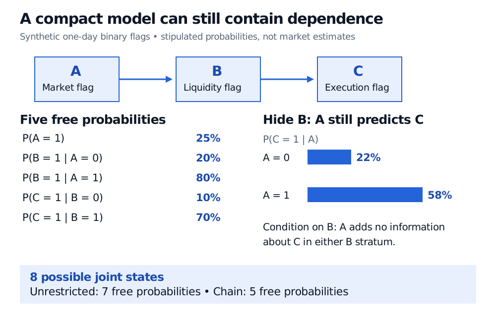
Consider three synthetic binary flags for one trading day: market flag A, liquidity flag B and execution flag C, with 1 denoting a flag. Stipulate the chain A→B→C and factorisation
p(a,b,c)=p(a)p(b∣a)p(c∣b).
Here p denotes probability mass at the displayed values. Three binary variables have 23=8 joint states. An unrestricted joint table needs seven free probabilities, since its eight entries sum to one. The chain needs five: one for A, two for B given the possible values of A, and two for C given the possible values of B. Each remaining binary probability is the complement of its row's specified probability. These counts assume unrestricted local Bernoulli tables, with no parameter tying.
Choose the following inputs:
Local probability
Value
p(A=1)
25%
p(B=1∣A=0)
20%
p(B=1∣A=1)
80%
p(C=1∣B=0)
10%
p(C=1∣B=1)
70%
All eight joint probabilities now follow from the factors. For example, the probability that all flags are one is 0.25(0.80)(0.70)=0.14, or 14%. This is the local-table storage principle described in Berkeley's Bayesian-network representation chapter.
Synthetic chain A to B to C has eight joint states and five free probabilities, versus seven unrestricted. Inputs are 25%, 20%, 80%, 10% and 70%. With B hidden, C has probability 22% given A=0 and 58% given A=1.
Original stipulated one-day flag model, not market estimates. Local conditional tables reduce the parameter count; the two bars show that hiding the middle flag leaves the endpoints dependent.
The saving comes from A⊥C∣B: once B is known, learning A adds no information about C. It does not imply marginal independence. Summing over the hidden liquidity flag gives
The market flag remains informative when liquidity is unobserved. “No direct edge” and “no association” are different claims. These are imposed probabilities, not evidence that the chain fits actual trading data.
Representation, inference and learning
Representation specifies the variables, factors and structural assumptions. Inference answers a query under that model, such as the probability of the execution flag given observed market information. Learning estimates parameters, or sometimes structure, from data. CMU's exact-inference notes separate these tasks.
Compact representation does not guarantee cheap inference. Intermediate factors can become large when variables are summed out. Belief propagation exploits local messages; sum-product is exact on a tree factor graph, while applying it around loops generally supplies an approximation. The graph is a model description, not an accuracy certificate for an inference algorithm.
Arrows also do not automatically establish causality. A directed factorisation describes an observational joint law; interpreting an intervention requires additional causal assumptions. An edge can permit dependence without forcing it for every numerical parameter choice. Nor must a graph display every extra independence that happens to hold for particular parameters.
For further worked teaching, Bayesian Networks and Markov Random Fields develops local structures, d-separation and clique potentials. Its preview is public; the full lesson requires membership.