Markov random field and factor graph: Definition & Examples

A Markov random field (MRF), also called a Markov network, represents a joint distribution with an undirected graph whose separations encode conditional independence. A factor graph displays the local functions whose product defines that distribution. For a quant researcher modelling interacting risk flags, the distinction separates two questions: which dependencies are allowed, and exactly how are joint outcomes scored?

Scores first, probabilities second

For finite discrete variables, a clique-factorised model has the form

p(x)=\frac{1}{Z}\prod_{C\in\mathcal{C}}\psi_C(x_C), \qquad Z=\sum_x\prod_{C\in\mathcal{C}}\psi_C(x_C).

A clique is a subset of variables with every pair joined. Each potential

\psi_C

is a non-negative compatibility score; it need not sum to one. The partition function

Z

normalises their product, and must satisfy

0<Z<\infty

. Unary factors score individual variables; pairwise factors score pairs. Larger cliques can support higher-order interactions. See Montanari §§1.2–1.4.

Consider two fictional binary risk flags, $A$ and $B$ . Let both unary factors be identically one, and set

\psi(a,b)= \begin{cases} 2,&a=b,\\ 1,&a\ne b. \end{cases}

This expresses a preference for matching flags without favouring zero over one.

State $(A,B)$	Unnormalised weight	Joint probability
$(0,0)$	2	$1/3$
$(0,1)$	1	$1/6$
$(1,0)$	1	$1/6$
$(1,1)$	2	$1/3$

The four weights sum to $Z=6$ , so

\mathbb{P}(A=B)=\frac{2+2}{6}=\frac23.

Each marginal probability of a flag equalling one is still

1/2

. Yet the probability of both equalling one is

1/3

, rather than the

1/4

obtained by multiplying the marginals. Learning

A=1

changes the probability of

B=1

2/3

. The interaction changes the joint law while leaving these individual flag rates unchanged. These are stipulated toy scores, not estimates of market co-movement.

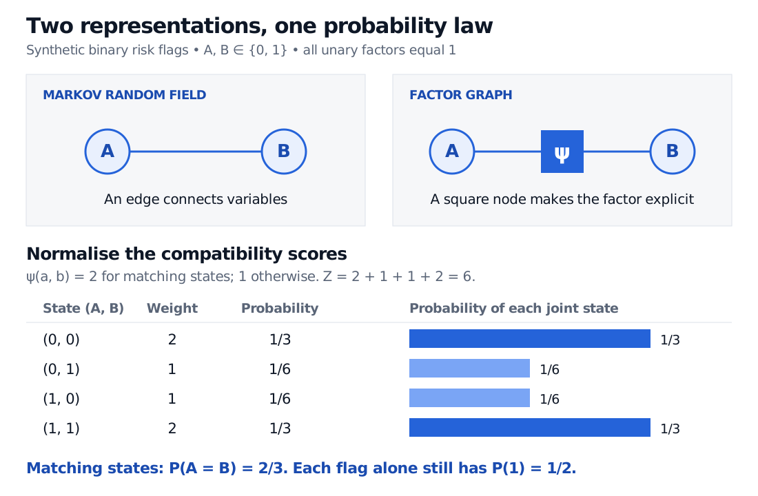
A two-node undirected graph A–B and a factor graph A–psi–B encode the same synthetic law. States (0,0), (0,1), (1,0), (1,1) have weights 2, 1, 1, 2 and probabilities one third, one sixth, one sixth, one third. Z is 6 and the probability of matching states is two thirds.

Original synthetic model. Adding a factor node changes the representation, while the four joint probabilities stay the same. Bar lengths show probabilities on one common scale.

What the factor node adds

The MRF draws an edge between

A

and

B

. Its factor graph instead draws two variable nodes and a square factor node for

\psi

, joined to both variables. Constant unary factors can be omitted. This is the same probability law, with the factorisation made explicit.

Factor graphs are bipartite: edges join variables to factors, and a variable connects to a factor exactly when it is an argument of that function. The distinction matters for a triangle: one three-variable factor and a product of three pairwise factors share the same complete MRF graph, but impose different factorisation structures. Sutton §2.1.1 explains this ambiguity. Factor nodes represent functions, not extra random variables or hidden market drivers.

A missing edge is a conditional statement

For an MRF, non-neighbours

X_i

and

X_j

are independent given all remaining variables. More generally, if a set

S

separates disjoint node sets

U

and

V

, then

X_U

and

X_V

are independent given

X_S

. Thus in a three-node chain

A-B-C

, conditioning on

B

separates the endpoints; their marginal independence is not guaranteed. An existing edge allows dependence but does not require it for every parameter choice.

The Hammersley–Clifford theorem makes the connection precise for finitely many finite-valued variables: if the joint mass is strictly positive at every point of the full Cartesian state space, the Markov properties and clique factorisation are equivalent. A valid non-negative clique factorisation implies the global separation property even with zeros, for conditioning events of positive probability. Without strict positivity, the reverse implication cannot be assumed. Chen's Lecture 5, “Hammersley-Clifford theorem” states the finite-state conditions.

An undirected edge supplies no causal direction. A Bayesian network instead uses a directed acyclic graph with normalised conditional distributions; causal interpretations still require additional assumptions.

A compact model can still be expensive

Evaluating the product for one configuration can be cheap while summing it over every configuration is costly. With

n

binary variables, brute-force normalisation visits

2^n

states. Graph structure can reduce that cost: sum-product message passing is exact on a tree factor graph, with manageable local state spaces and factor sizes. On graphs with loops, ordinary loopy belief propagation has no general guarantee of convergence or exact marginals. See Montanari §§2.2–2.3 and Sutton §2.1.3.

For the broader comparison, Bayesian Networks and Markov Random Fields develops clique structure, separation and directed alternatives. Its preview is public; the full lesson requires membership.

Sources

Andrea Montanari, Inference in Graphical Models (2011), §§1.2–1.5 and 2.2–2.3: pairwise factors, partition functions, factor graphs and tree versus loopy inference.
Yen-Chi Chen, UW STAT 535, Lecture 5: Graphs and Networks: Markov properties, factorisation and the positivity condition in the finite-state Hammersley–Clifford theorem.
Charles Sutton, Efficient Training Methods for Conditional Random Fields (2008), §§2.1.1–2.1.3: factor-graph representation, ambiguity of MRF factorisations and inference complexity.

Scores first, probabilities second

What the factor node adds

A missing edge is a conditional statement

A compact model can still be expensive

Sources

Related terms

Bayesian network

Belief propagation

Conditional independence

Joint distribution

Marginal distribution