How sum-product messages compute marginal probabilities on trees, why loops change the guarantee, and how max-product differs from marginal inference.
Belief propagation
Belief propagation (BP) is a message-passing algorithm for inference in a probabilistic graphical model. Its sum-product form computes exact marginal probabilities on a tree by combining local factors and reusing partial sums. In a quant model with unobserved market states, this can turn an otherwise enormous sum over possible state configurations into small local calculations. Exact inference is still conditional on the model: it does not establish that the chosen states or dependencies describe markets correctly.
The nonnegative unary factors ϕi encode local evidence or preferences; the pair factors ψij encode compatibility. The normaliser Z makes the joint probabilities sum to one, and must be positive and finite. A factor need not itself be a probability distribution. A factor graph represents each factor separately from its variables; the expression above uses the convenient pairwise-node notation.
For neighbour set N(i), the sum-product message from i to j is a function of the receiver’s state:
Multiply the evidence arriving from the other neighbours, include the local and pair factors, then sum out xi. Excluding j prevents immediately sending its own information back. On a tree, the message summarises the entire sender-side subtree. The marginal distribution at j follows from
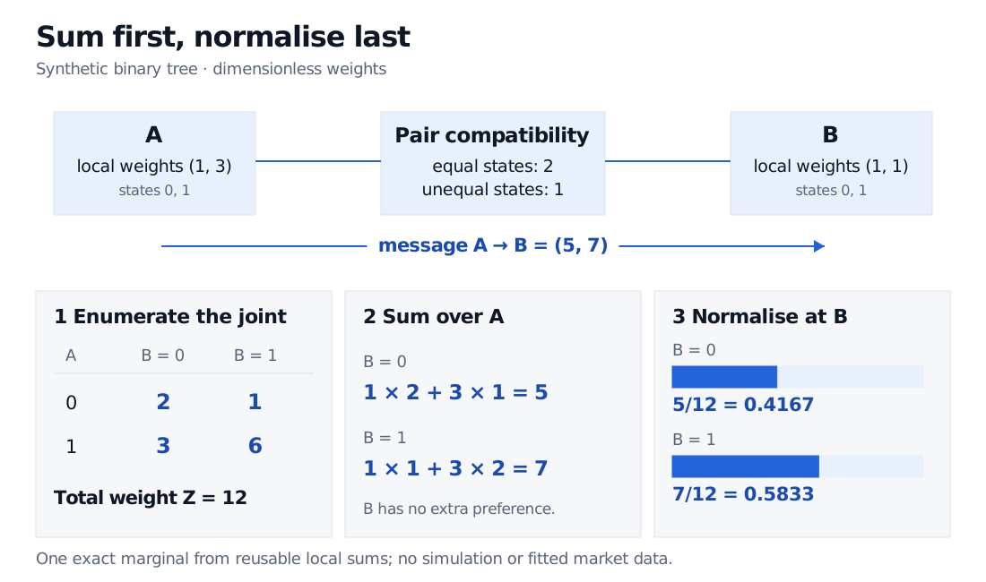
Let A,B∈{0,1}. Stipulate ϕA(0)=1, ϕA(1)=3, and ϕB(0)=ϕB(1)=1. Set ψ(a,b)=2 when the states agree and 1 otherwise. These are fictional, dimensionless weights, not estimated financial probabilities.
There are no other neighbours, so the incoming-message product at A is the empty product, equal to one:
mA→B(0)mA→B(1)=1×2+3×1=5,=1×1+3×2=7.
Because B has a constant unary factor, its probabilities are p(B=0)=5/12 and p(B=1)=7/12. The message itself is (5,7); it is not yet a probability vector.
An independent check enumerates the joint weights:
A
B
Unnormalised weight
0
0
2
0
1
1
1
0
3
1
1
6
Their total is Z=12. Summing the rows with B=0 gives 2+3=5; the other rows give 1+6=7. BP has organised the same marginalisation into a message.
Synthetic two-node binary tree: joint weights for states (0,0), (0,1), (1,0), (1,1) are 2, 1, 3, 6. Summing over A gives message (5,7) to B. Normalising by 12 gives B probabilities 5/12 and 7/12.
Original synthetic example. The two entries of a message index the receiving node’s states; they are weights until normalised.
A message may be multiplied by a positive constant independent of its state without changing the final normalised marginal. For example, sending (5/12,7/12) here produces the same answer as sending (5,7). Message normalisation helps control numerical scale; a message is not generally the full marginal at either endpoint. See Foundations of Computer Vision, §29.7.1.
Why a tree is a substantive assumption
On a finite tree, removing an edge separates two subtrees. Their summaries can be combined without overlapping information, using the model’s conditional independence. A pass toward a chosen root and a pass back outward give all node marginals exactly. Mézard and Montanari, §14.2 and Theorem 14.1 formalise this property. Factor sizes and variable state spaces still determine the cost of each local calculation.
With cycles, loopy belief propagation repeats the local updates. Evidence can return along another path; simply excluding the recipient does not eliminate that effect. The procedure need not converge, and stable messages need not yield exact marginals. Stanford CS228’s notes, Fact 105 state both limits explicitly. Check convergence separately from accuracy; compare against exact enumeration on small versions of the model when feasible.
For a financial application, a chain of latent regimes is structurally different from a dense network of interacting issuers. Efficient exact inference for the chain does not establish an exactness guarantee for the network. Likewise, estimating a historical latent state using later observations is smoothing; using that estimate in a trading decision dated before those observations would introduce future information. These are model and information-set choices, beyond the message-update arithmetic.
Marginals and the most likely configuration answer different questions
Sum-product adds probability mass across alternatives. Max-product replaces the sum with a maximum, producing max-marginal scores. On a tree, retaining compatible maximising choices and tracing them back recovers a joint maximum a posteriori estimate. This is distinct from selecting the most probable state independently from each sum-product marginal. See CMU’s exact-inference notes, “Message Passing Algorithms”.
In the worked model, max-product sends (3,6) to B, whereas sum-product sends (5,7). The joint maximum is (A,B)=(1,1) with weight 6. Normalising max-product scores does not turn them into marginal probabilities.
Ties make compatible traceback especially important. In a separate two-node model with constant unary factors, give unequal states weight 4 and equal states weight 1. Both states of either node have max-marginal score 4. Independently breaking both ties toward zero selects (0,0) with weight 1, even though (0,1) and (1,0) each have weight 4. Local maximising choices must fit together.