Bayesian network: Definition & Examples

A Bayesian network represents a joint probability distribution using a directed acyclic graph and a conditional distribution for each variable given its parents. Its missing arrows encode assumptions about conditional independence. For a quant researcher, that makes the graph a compact specification of which risks or signals can share information, and which relationships the model rules out.

A network can describe stress indicators, defaults or diagnostic signals without storing a separate unrestricted probability for every possible joint outcome. The saving comes from independence assumptions, so choosing a sparse graph is a substantive modelling decision.

What the arrows buy you

A parent is a node with an arrow directly into another node. Acyclic means that following arrow directions cannot return to the starting node. For variables

X_1,\ldots,X_n

, the network specifies

p(x_1,\ldots,x_n)=\prod_{i=1}^{n}p\bigl(x_i\mid x_{\mathrm{pa}(i)}\bigr),

where

\mathrm{pa}(i)

denotes the parents of node

i

. A root node contributes its unconditional distribution. Discrete variables use probability tables; continuous variables need suitable conditional densities or other distributional specifications. Each local distribution must be normalised. This factorisation defines the full joint law, rather than only a collection of pairwise associations. Berkeley CS188 §6.3 develops this representation.

The word Bayesian does not require a prior distribution over every table entry. The network may have probabilities supplied by experts or estimated from data, including by maximum likelihood. Bayesian parameter inference is an additional choice. Poole and Mackworth §10.4 explains learning the conditional distributions when the graph is supplied.

Two flags can cluster without a direct arrow

Consider a fictional fixed-horizon risk model. Let $C=1$ denote a stress regime, and let $A=1$ and $B=1$ denote two risk flags. Use the fork $A\leftarrow C\to B$ and assume the flags are independent given either value of $C$ :

p(c,a,b)=p(c)\,p(a\mid c)\,p(b\mid c).

Set $\mathbb{P}(C=1)=0.20$ , with these conditional probabilities:

Regime	$\mathbb{P}(A=1\mid C)$	$\mathbb{P}(B=1\mid C)$
$C=0$	0.10	0.05
$C=1$	0.80	0.60

The probabilities for a flag equalling zero are the complements. Marginalising over the regime gives

\mathbb{P}(A=1)=0.24

and

\mathbb{P}(B=1)=0.16

. But the joint probability is

\begin{aligned} \mathbb{P}(A=1,B=1) &=0.20(0.80)(0.60)+0.80(0.10)(0.05)\\ &=0.096+0.004=0.10. \end{aligned}

Multiplying the marginals instead gives

0.24\times0.16=0.0384

. Thus the flags are dependent in the mixed population even though they are independent within each regime. The missing edge between

A

and

B

does not assert marginal independence. The unobserved shared regime carries their association.

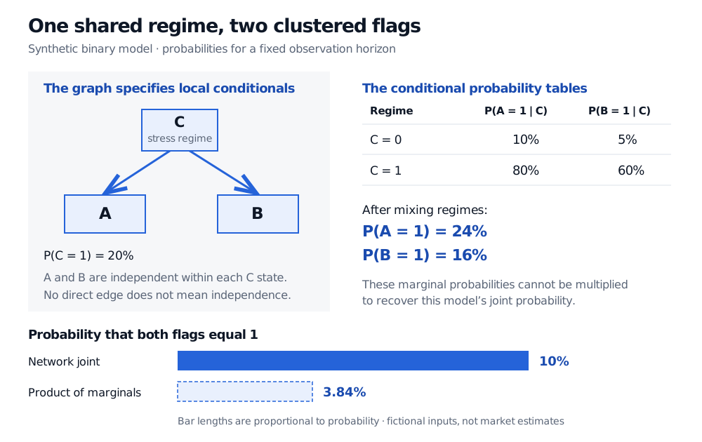
A synthetic fork sends C to A and B, with stress-regime probability 20 percent. Flag probabilities are 80 and 60 percent in stress, versus 10 and 5 percent otherwise. Their joint probability is 10 percent, compared with 3.84 percent from multiplying the marginals.

Original synthetic model. The graph and tables produce a 10% probability of both flags, while the product of marginal probabilities is 3.84%. The bar lengths are proportional to probability; inputs are not market estimates.

Inference can run against the arrows. If both flags are observed, Bayes' theorem gives

\mathbb{P}(C=1\mid A=1,B=1)=\frac{0.096}{0.10}=0.96.

The network's stress probability moves from 20% to 96% after this evidence. That is a consequence of the stipulated tables, not evidence that real flags identify stress with this accuracy. If the regime is hidden, conditional independence must still be justified; it does not follow from simply giving the hidden node a name.

D-separation: which paths remain open?

D-separation reads conditional independencies from the graph. Consider paths without requiring travel to follow arrow directions. A path is blocked when it contains either an observed non-collider, or a collider for which neither that node nor any descendant is observed. A collider has two arrowheads meeting at it. If every path between two nodes is blocked by the conditioning set, the nodes are conditionally independent under the network.

The three basic motifs explain why conditioning can have opposite effects:

Isolated three-node graph	What conditioning on the middle node does
Chain: $A\to C\to B$	Blocks the path; the endpoints become conditionally independent.
Fork: $A\leftarrow C\to B$	Blocks the path, as in the regime example.
Collider: $A\to C\leftarrow B$	Opens the path; initially independent endpoints can become dependent. Observing a descendant of $C$ can also open it.

Larger graphs require checking all paths. An open path means independence is not guaranteed by the structure; particular probability choices can still create additional independence. See Poole and Mackworth §11.1.2 and Berkeley CS188 §6.5.

Representation is not causal identification

An arrow specifies which variables enter a local conditional distribution. It does not, by itself, prove what an intervention would change. A causal interpretation adds assumptions about mechanisms and the adequacy of the variables and graph. Observing a risk flag and forcing that flag to change are different questions. Poole and Mackworth §11.1 distinguishes observational inference from intervention explicitly.

A naive Bayes classifier is a special network with the class as parent of each feature and conditional independence among those features. General Bayesian networks allow richer structures. A small graph can simplify storage without making every inference query cheap; the pattern of connections matters for computation.

For the probability foundations behind the example, Joint Distributions and Dependence develops marginalisation and independence tests. Its preview is public; the full lesson requires membership.

Practice: selecting on a collider

Two binary risk triggers $U$ and $V$ are independent, each with probability $1/2$ of equalling one. A case is selected exactly when at least one trigger equals one: $S=1$ if $U=1$ or $V=1$ . Are the triggers independent among selected cases?

Answer. No. The four input pairs are equally likely, and selection retains only

(1,0)

(0,1)

and

(1,1)

. Within the selected cases, each trigger has probability

2/3

of equalling one, but both equal one with probability

1/3

, which differs from

4/9

. Conditioning on the collider

U\to S\leftarrow V

creates dependence in this example. Once selected, learning that one trigger is absent makes the other certain to be present.

Sources

UC Berkeley CS188, §6.3: Bayesian Network Representation: graph structure, conditional tables and joint factorisation.
UC Berkeley CS188, §6.5: D-Separation: chain, fork, collider and path-based independence guarantees.
David Poole and Alan Mackworth, Artificial Intelligence: Foundations of Computational Agents, 3rd ed., §11.1: causal mechanisms, interventions and d-separation, including extra independencies due to particular parameter values.
Poole and Mackworth, §10.4: Learning Belief Networks: expert-supplied versus learned probabilities, fixed structure and hidden variables.

What the arrows buy you

Two flags can cluster without a direct arrow

D-separation: which paths remain open?

Representation is not causal identification

Practice: selecting on a collider

Sources

Related terms

Bayes' theorem

Conditional independence

Joint distribution

Marginal distribution

Naive Bayes classifier