Find the inputs that make a polynomial zero, distinguish break-even sizes from a profit maximum, and interpret repeated, real and complex roots.
Polynomial root
A polynomial root is an input r that makes a polynomial equal zero: p(r)=0. It is also called a zero of the polynomial. For a real root, the graph of y=p(x) meets the horizontal axis at (r,0).
The root is the inputr; zero is the resulting output. In a profit model, a root can identify a break-even position size. It does not, by itself, identify the most profitable size.
Two break-even sizes
Consider an original, hypothetical sizing model. Let q≥0 be a continuous trading quantity, measured in abstract units, and let net profit be
Π(q)=−q2+10q−16USD.
The coefficients have units: the quadratic cost coefficient is USD 1 per quantity-unit squared, the linear contribution is USD 10 per quantity-unit, and the fixed setup cost is USD 16. The model assumes these coefficients remain constant; it is a teaching example, not an estimate of actual execution costs or trading returns.
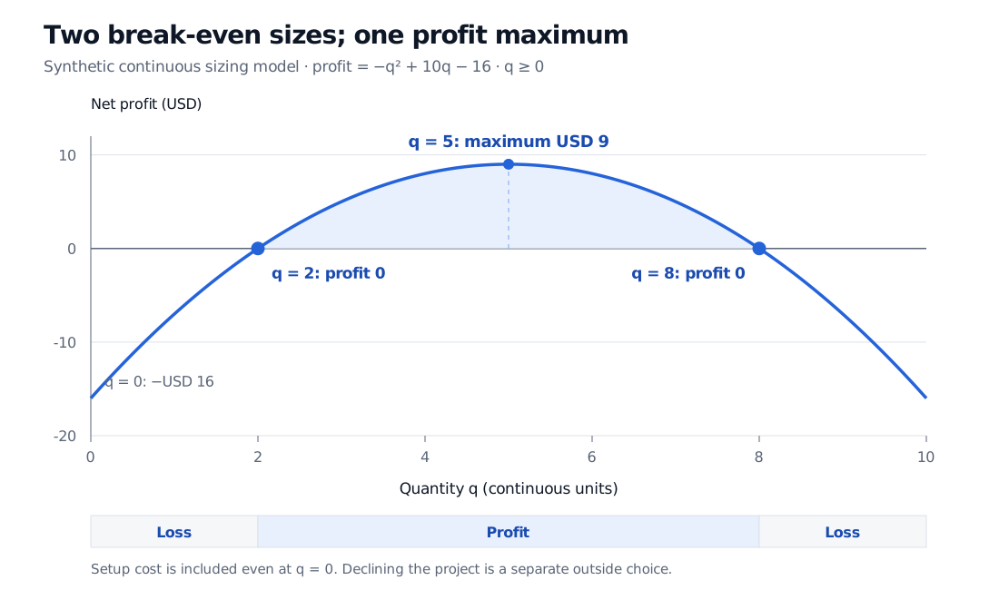
Setup has been incurred within this model, so Π(0)=−16: zero quantity still bears the fixed cost. A choice to decline the project before paying setup would need a separate outside payoff. It is not represented by setting q=0 in this formula.
Break-even requires Π(q)=0. Factorising gives
−q2+10q−16=−(q−2)(q−8).
A product is zero when at least one factor is zero, so the roots are q=2 and q=8. Substituting into the original expression checks both:
Π(2)=−4+20−16=0,Π(8)=−64+80−16=0.
Both roots satisfy the quantity restriction. If a model required a different domain, such as a capacity bound or whole units, that restriction would be applied to the mathematical solutions before using them.
The factors also reveal where profit changes sign:
Quantity
Signs of (q−2) and (q−8)
Net profit
0≤q<2
Both negative
Negative
2<q<8
One positive, one negative
Positive
q>8
Both positive
Negative
The leading minus sign reverses the sign of the product. Increasing size past the first root initially makes the project profitable, but increasing it beyond the second root makes the quadratic cost dominate.
Synthetic net profit in USD equals minus q squared plus ten q minus sixteen. It is zero at quantities 2 and 8, positive between them, and maximised at quantity 5 with profit USD 9. At zero quantity, the incurred setup cost leaves profit minus USD 16.
Original synthetic continuous-quantity model. The two roots mark zero profit; the peak marks a different decision. The fixed USD 16 setup cost is included at every quantity.
To locate the maximum, complete the square:
Π(q)=9−(q−5)2.
The squared term is non-negative, so profit cannot exceed USD 9, attained at q=5. This is an optimisation question. Solving Π(q)=0 answers the break-even question instead. Equivalently, the derivativeΠ′(q)=10−2q is zero at the peak, not at either break-even size.
A root can touch without crossing
The factor theorem connects a root to an algebraic factor: p(r)=0 if and only if x−r divides p(x) without a remainder. A repeated factor gives a root its multiplicity. More precisely,
p(x)=(x−r)mg(x),g(r)=0,
means that r has multiplicity m.
For real polynomials, an odd multiplicity changes the sign across the root; an even multiplicity does not. For example, (x−3)2 is zero at 3 and positive on either side: its graph touches the axis and turns back. By contrast, (x−3)3 crosses the axis, even though it has a horizontal tangent there. A flat tangent does not establish whether the sign changes. OpenStax §5.3 develops this relationship between multiplicity and graph shape.
This matters for numerical root-finding: searching only for intervals with opposite endpoint signs can miss an even-multiplicity root. In the sizing example, both roots have multiplicity one, and profit crosses zero at each.
Real roots, complex roots and usable answers
A nonzero polynomial of degree n has at most n distinct roots. Over the complex numbers, a degree-n polynomial has exactly n roots counting multiplicity. Those need not be real: x2+1 has roots i and −i, but no real horizontal-axis intercepts. Constant nonzero polynomials have no roots; the identically zero polynomial is a separate case for which every input is a root. See OpenStax §5.5 for the factorisation results.
A complex root cannot serve as a real trading quantity. Even a real root must satisfy the model's units, domain and economic interpretation. Algebra finds the zeros; the model determines which zeros answer the financial question.
For more work with equations, the Mathematics Primer's algebra lesson connects linear and quadratic equations to break-even sizing and shows how quantity restrictions can change a usable answer. The full lesson requires membership; a public preview is available.
Sources
James Stewart, Single Variable Calculus: Early Transcendentals, 6th edition, §1.2 (polynomials and quadratic models), §4.8 (numerical roots), and Appendix H (complex roots).