Complex number

For a quant, complex numbers become useful when a model's probability distribution is easier to describe through oscillations than through a density. Fourier transforms and characteristic functions use them to package sine and cosine information together. The resulting option price is still a real cash amount.

A point, a length and an angle

For $z\ne0$, choose an angle $\theta$ from the positive real axis, measured counterclockwise in radians. Then

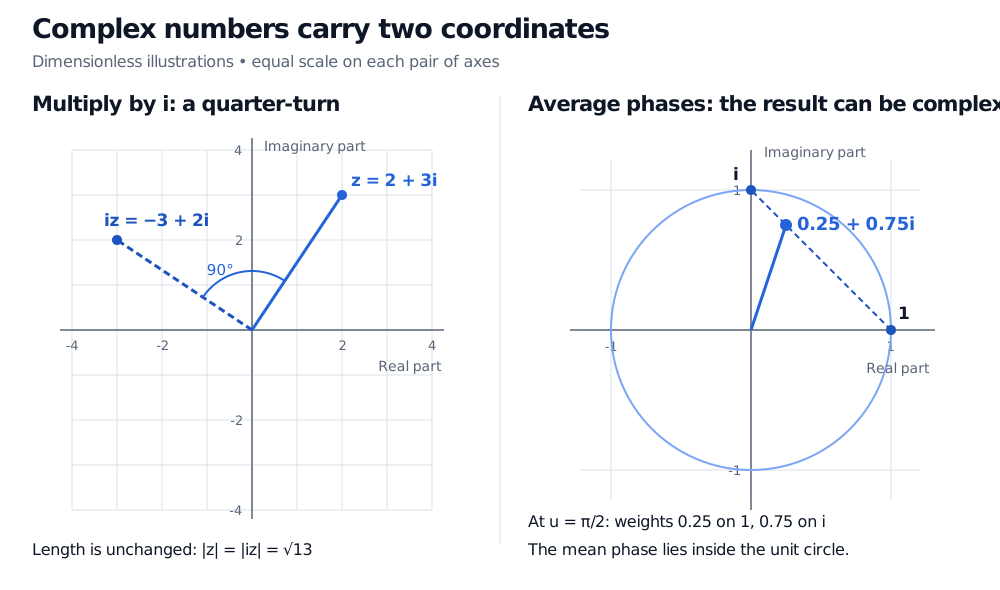
Multiplication by $i$ sends $(a,b)$ to $(-b,a)$: a counterclockwise quarter-turn with no change in length. Thus $2+3i$ becomes $-3+2i$. More generally, multiplying nonzero complex numbers multiplies their lengths and adds their angles, modulo whole turns. This is why complex exponentials suit waves and frequency calculations.

Arithmetic without a new rulebook

Addition combines coordinates. Multiplication expands brackets as usual, with $i^2$ replaced by $-1$:

For example,

The positive $6$ in the real part is the crucial sign: $-6i^2=+6$. Multiplying real parts and imaginary parts separately would miss the cross terms.

In general, $(c+di)(c-di)=c^2+d^2$, so the denominator becomes real and positive unless $c=d=0$. Division by zero remains undefined.

There is no usual greater-than ordering on complex numbers compatible with field arithmetic. A pricing routine cannot ask whether a complex payoff is “positive” in the same way it uses $\max(S_T-K,0)$ for a real call payoff. Modulus compares lengths; it does not turn a complex intermediate value into a cash price.

A real payoff with a complex transform

Now encode the same two-outcome distribution using its characteristic function. For a real frequency $u$, with $uX$ measured in radians,

At $u=\pi/2$, the two possible phase values are $1$ and $i$, so

Every phase $e^{iuX}$ has unit modulus for real $u$ and real $X$. Averaging those phases can shorten the resulting vector, explaining $\lvert\phi_X(u)\rvert\le1$. It need not lie on the unit circle, even though each outcome's phase does. Nor can one generally replace $\mathbb{E}[e^{iuX}]$ with $e^{iu\mathbb{E}[X]}$: averaging and applying the exponential are different operations.

How the complex part disappears from a price

For a real-valued random variable and real $u$,

The negative-frequency transform has the same real part and the opposite imaginary part. In a valid Fourier inversion, this symmetry pairs contributions so that imaginary terms cancel; equivalent half-axis formulas explicitly take a real part. Inversion still needs its convergence conditions. Our discrete indicator example illustrates the encoding directly; it is not a continuous-density inversion example.

A small imaginary residue in a calculation whose exact result is real can arise from numerical error. A material residue calls for checks of transform conventions, integration accuracy and any complex logarithm or square-root branches. Taking a real part indiscriminately does not validate an incorrect formula.

Sources

• Sheldon Axler, Linear Algebra Done Right, 2nd edition, Chapter 1, “Complex Numbers,” pp. 2–3 — complex-number definition and arithmetic.
• MIT OpenCourseWare, ES.1803 Differential Equations, Spring 2024, Class 6: Complex Numbers, §§4–5 — complex plane, Euler's formula and polar representation.
• Jim Gatheral, The Volatility Surface: A Practitioner's Guide (Wiley, 2006), Chapter 5, pp. 56–57 — characteristic-function representations in financial models.
• Peter Carr and Dilip B. Madan, “Option valuation using the fast Fourier transform”, Journal of Computational Finance 2(4), Summer 1999, pp. 61–73, §§2–3 — risk-neutral characteristic functions and recovering real option values through Fourier methods.