Polychoric correlation estimates latent Gaussian dependence behind ordered categories; tetrachoric is its binary case. A threshold example separates latent rho 0.7071 from binary phi 0.5.
Polychoric and tetrachoric correlation
Polychoric correlation estimates the correlation between two unobserved continuous variables, assuming a bivariate normal distribution whose thresholds generate the observed ordered categories. Tetrachoric correlation is the special case in which both observed variables are binary. For a quant analysing ordered risk assessments or investor survey responses, the distinction matters: correlation between the category codes answers a different question from correlation between the assumed latent variables.
Factor analysis of ordinal responses is one application. A latent-variable interpretation must be meaningful for the measurement process; assigning numbers to unordered labels does not create an ordered scale.
The cutpoints increase strictly, with a0=b0=−∞ and ar=bc=+∞. Fixing both latent means to zero and variances to one sets their location and scale: the category table cannot identify arbitrary latent units. The target ρ is Pearson correlation on this stipulated latent scale, rather than on the observed category codes.
where Φ2 is the bivariate standard normal cumulative distribution function. These probabilities must be nonnegative and sum to one. Changing a category's numerical label while preserving its order leaves this model unchanged; changing the category boundaries changes the information observed.
Stipulate ρ=0.5≈0.7071 and cut both latent variables at zero:
X=1{Z1>0},Y=1{Z2>0}.
Both indicators have probability 1/2 of being 1. In this balanced Gaussian case, the upper-right quadrant probability is
q=P(X=1,Y=1)=41+2πarcsin(ρ)=83=0.375.
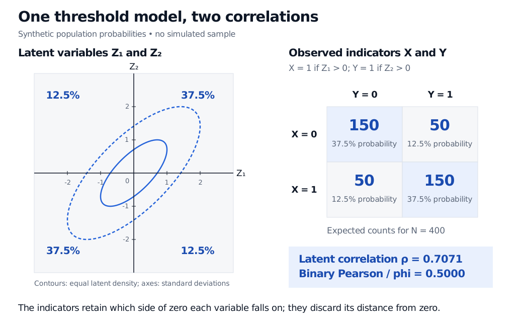
Symmetry gives the following synthetic population table, alongside expected counts for N=400 independent pairs. These are model expectations, not a simulated or empirical dataset.
Observed pair
Probability
Expected count
X=0,Y=0
0.375
150
X=0,Y=1
0.125
50
X=1,Y=0
0.125
50
X=1,Y=1
0.375
150
Total
1.000
400
The binary Pearson coefficient, also called phi, is
The indicators retain the signs of Z1 and Z2 but discard their distances from zero. Their correlation of 0.5 is a correct description of the binary outcomes. Under the stated threshold model, the latent correlation is 0.7071.
Synthetic standard bivariate normal model with latent correlation 0.7071 cut at zero on both axes. Matching-sign quadrants each have probability 37.5%, opposing-sign quadrants 12.5%. Expected counts at N equals 400 are 150, 50, 50, 150; binary Pearson correlation is 0.5000.
The same stipulated Gaussian model produces two different correlation coefficients. Contours show equal latent density; table counts are expectations for 400 independent pairs.
Combining the two displayed equations yields
ϕ=π2arcsin(ρ),ρ=sin(2πϕ).
This shortcut requires both zero thresholds and the Gaussian model. Unequal category frequencies require their own cutpoints and rectangle probabilities. In credit modelling, the same distinction separates default-indicator correlation from latent credit-quality correlation; the balanced 50% illustration above is not a default-rate calibration.
For the covariance arithmetic behind phi, Expectation, Variance and Covariance develops the calculation from probability weights (free signed-in account required; public preview available).
up to a constant. Full ML estimates the thresholds and correlation together. A common two-step method first obtains marginal cuts, for example
ai=Φ−1(N∑k=1i∑j=1cnkj),
then holds the cuts fixed while numerically optimising over ρ. Here Φ−1 is the standard normal quantile function. In the balanced example, each cut is Φ−1(0.5)=0. If the expected counts above were instead an actual observed table, both fitting approaches would return approximately 0.7071.
The official polycor manual, “polychor”, documents both estimators. It also states that its two-step standard error treats estimated thresholds as fixed; that uncertainty calculation differs from joint ML's parameter covariance. Report the method, sample size and uncertainty alongside the coefficient. The example's exact population probabilities do not imply that a sample estimate has no sampling error.
A fitted number is conditional on the model
A strictly positive two-by-two table has three independent proportions; the tetrachoric model has two cutpoints and one correlation. It is exactly identified. A perfect fit to that table therefore supplies no spare restriction with which to validate latent normality. More ordered categories can supply restrictions to assess fit, but cannot reveal the full unobserved distribution without assumptions. If the latent joint law is not Gaussian, the fitted coefficient need not equal its actual Pearson correlation. A fitted latent correlation is not a causal effect.
Sparse cells can make estimation unstable; extreme tables can put the optimum at a singular correlation boundary. A numerical cap below ∣ρ∣=1 is a computation safeguard, not evidence that the estimate is precise. A constant variable provides no usable correlation information. Any adjustment to zero counts must be reported because it changes the fitted table.
Across many variables, separately fitted pairwise correlations may fail to form a positive semidefinite matrix. The Stata tetrachoric manual discusses both zero-count adjustments and matrix repair. Such repair changes the estimates; it does not establish a valid common latent model.
Finally, polyserial correlation concerns one continuous and one ordinal variable. It is a different measurement setup from the two ordinal variables used for polychoric correlation.