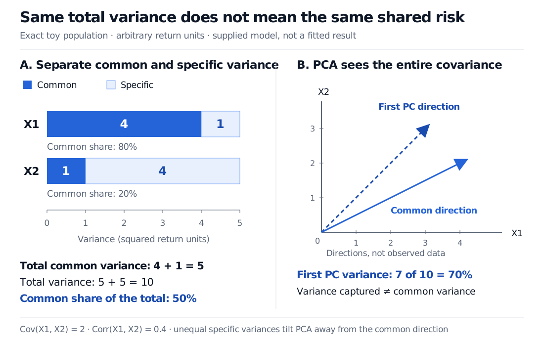
Factor analysis models shared covariance through latent factors and separates specific variance. A two-variable example shows why it differs from PCA.
Factor analysis
Factor analysis is a statistical model that explains co-movement among observed variables using a smaller set of unobserved, or latent, factors, while allowing each variable its own specific variance. In quantitative finance, that separation can turn a large return covariance matrix into a common-risk component plus a diagonal specific-risk component. A good fit describes dependence; it does not establish what economically caused the returns.
What the model separates
For a centred vector of p variables, write
x=Λf+ε,Cov(f)=Ik,Cov(ε)=Ψ.
Here k<p, Λ is the loading matrix, and Ψ is diagonal with nonnegative entries. Take factors and errors to have zero means, and assume they are uncorrelated with each other. The resulting covariance is
Σ=ΛΛ⊤+Ψ.
The first term supplies all cross-variable covariance; the second supplies variable-specific variance. In the Gaussian version, the factors and errors are independent normal vectors, giving x∼N(0,Σ). The covariance identity itself only needs the stated second-moment restrictions, not normality. Ng's factor-analysis notes develop this generative model.
A variable's communality is its common-factor variance: the corresponding diagonal entry of ΛΛ⊤. Its uniqueness is the corresponding entry of Ψ. For standardized variables these sum to one, so communality is also a share of total variance. For variables on other scales, divide common variance by total variance to obtain that share. “Specific” means unexplained by these factors; it need not mean measurement error or economically irrelevant noise. UCLA’s variance-partitioning discussion distinguishes unique variation from measurement error.
Two equally volatile series, different shared risk
Consider an exact, fictional population model for centred return-like measurements in arbitrary units:
X1=2F+ε1,X2=F+ε2,
where F∼N(0,1), ε1∼N(0,1) and ε2∼N(0,4) are mutually independent. Then
Σ=(4221)+(1004)=(5225).
Both series have variance 5, measured in squared return units. But their common variances are 4 and 1: the shared factor accounts for 80% of the first series' variance and 20% of the second's. Their covariance is 2×1×Var(F)=2, while their correlation is only 2/5×5=0.4. Sharing the same factor does not imply perfect correlation when specific variance remains.
Exact toy model: X1 has common variance 4 and specific variance 1; X2 has common variance 1 and specific variance 4. Both totals are 5 and their correlation is 0.4. The common direction has slope 0.5, while the first principal component has slope 1 and captures 70% of total variance, compared with a 50% total common-variance share.
Supplied toy population, not an estimate from market data. Unequal specific variances make the first PCA direction differ from the common loading direction; its explained-variance percentage answers a different question.
These loadings and specific variances were supplied, not recovered from the two-variable covariance matrix. Indeed, loadings 2 and 2 with specific variances 3 and 3 produce the same Σ. Two observed variables do not identify this unrestricted one-factor decomposition, even after fixing the factor variance to one. The example teaches covariance accounting, not unique factor discovery.
Why PCA gives a different answer
Ordinary principal component analysis (PCA) finds orthogonal directions that successively maximize variance of projections of the observed data. It uses total variance, without separately estimating a diagonal uniqueness matrix. Factor analysis instead models shared covariance and variable-specific variation. PCA can help initialize an analysis, but retaining principal components is not the same estimation problem. Ng's PCA notes derive the maximum-variance objective.
In this example, the first principal direction is (1,1)⊤/2, with variance 7; the other direction has variance 3. The first PC therefore captures 7/(7+3)=70% of total variance. Under the supplied factor model, common variance totals 4+1=5 out of 10, or 50%. Neither percentage contradicts the other: a PCA projection can retain specific variation as well as common variation.
The supplied common component lies along (2,1)⊤, whereas the first PC lies along (1,1)⊤. Unequal specific variances change the total-covariance eigenvectors. Reading the first PC as the original latent factor would miss that distinction.
Fitting factors does not fix their identity
In ordinary Gaussian maximum-likelihood factor analysis, choose a factor dimension, then estimate loadings and uniquenesses by the marginal likelihood; EM is one fitting approach. Factor scores are subsequent estimates of unobserved factor values. They are not directly observed returns. The R factor-analysis documentation distinguishes the specified factor count, likelihood fit and optional score estimators.
Even with adequate identification restrictions, factor coordinates need conventions:
Sign: replacing a factor and its loading column by their negatives leaves the common component unchanged.
Scale: multiplying a factor by a nonzero constant and dividing its loadings by that constant changes neither fitted observations nor covariance when its variance is adjusted consistently. Fixing factor variance to one removes this scale freedom.
Orientation: with identity factor covariance, any orthogonal Q gives equivalent loadings ΛQ and factors Q⊤f. Their product and implied covariance are unchanged. Factor rotation chooses a more interpretable representation; an economic label requires additional evidence.
For a financial application, inspect residual cross-covariances, sensitivity to the factor count and sample window, and stability outside the fitting period. A latent covariance factor is not automatically a traded portfolio, a priced risk factor, or a causal mechanism. Diagonal specific covariance is a modelling restriction that omitted common drivers can violate. Near-zero estimated uniquenesses also deserve scrutiny, as the R documentation's discussion of boundary solutions emphasizes.
For the portfolio calculation, Sections 3.2 and 3.4 of the SelfMadeQuant lesson Risk Models: APT and Factor Structure develop common and specific contributions to portfolio variance. The lesson Principal Component Analysis and the SVD View derives PCA's projection objective. Both have public previews; full lessons require membership.