How orthogonal random forests combine local forest weights and nuisance fitting, what the residual moment estimates, and why causality and inference require additional assumptions.
Orthogonal random forest
An orthogonal random forest (ORF) combines forest-based local weighting with Neyman-orthogonal estimating equations to estimate a parameter that varies with observed features while limiting first-order sensitivity to estimated nuisance functions. A quant might use it to study whether an execution intervention has different effects across liquidity conditions, controlling for a larger collection of recorded order characteristics. The original method is due to Oprescu, Syrgkanis and Wu (2019).
A local effect, with more controls than effect features
Separate two jobs for the covariates. Let X contain the features along which the effect is allowed to vary; let W contain additional pre-treatment controls. In a fictional execution study, X could describe liquidity, while W records characteristics affecting both the chosen intervention and the outcome. A good outcome predictor need not be a good estimator of the intervention's effect.
For a scalar treatment D and outcome Y, consider the restricted partially linear model
Y=θ0(X)D+f0(X,W)+ε,E[ε∣D,X,W]=0.
Here the treatment slope depends on X, but does not vary further with W at fixed X. With binary treatment and the causal assumptions below, it represents a conditional average treatment effect. For a continuous treatment, this model imposes a linear treatment response at each X; the coefficient is not an unrestricted dose-response curve. This specification is a useful case of the ORF framework, described in the EconML forest-method guide.
Write the nuisance conditional means as q0(X,W)=E[Y∣X,W] and g0(X,W)=E[D∣X,W]. Subtracting them gives outcome and treatment residuals. Around a target x, local nuisance fits produce
Yi=Yi−qx(Xi,Wi),Di=Di−gx(Xi,Wi).
For nonnegative forest weights αi(x) summing to one, the scalar local moment and its solution are
The denominator must be positive. This is a weighted regression through the origin after residualisation; adding an intercept changes the stated calculation. The EconML guide also explains local-linear corrections used by its implementation; the expression here illustrates the simpler local-constant moment.
Two residuals reveal what the moment does
Suppose D is a binary intervention indicator and Y an execution-improvement score in basis points, with higher values better. At one target feature value, stipulate these two residuals and equal local weights:
Observation
Treatment residual
Outcome residual (bp)
Local weight
Weighted cross-product (bp)
Weighted treatment square
A
−0.5
−1.0
0.5
0.250
0.125
B
+0.5
+1.5
0.5
0.375
0.125
Total
1.0
0.625
0.250
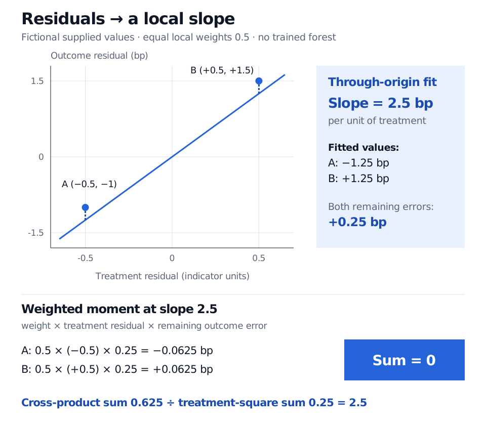
Thus θ(x)=0.625/0.25=2.5 bp per unit of the treatment indicator. At that slope, the two outcome residuals minus fitted values are both 0.25 bp. Their contributions to the estimating moment are −0.0625 and +0.0625 bp, which cancel. A zero weighted moment does not mean every fitted residual is zero.
Stipulated treatment residuals minus 0.5 and plus 0.5 have outcome residuals minus 1 and plus 1.5 basis points. Equal weights give a cross-product sum of 0.625 and treatment-square sum of 0.25, hence slope 2.5. The weighted moment contributions are minus 0.0625 and plus 0.0625.
Original fictional arithmetic example. The residuals and weights are supplied; no forest or nuisance model has been trained and no causal effect has been identified.
The positive slope says how these supplied residuals line up under the specified equation. Two rows cannot establish an intervention's benefit, provide a standard error, or verify that the controls are sufficient.
Where the forest and orthogonality enter
In ORF, shared tree leaves determine adaptive neighbourhood weights. Local nuisance fitting focuses on the region around the target x, rather than only optimising overall prediction error. The original construction incorporates nuisance estimation into splitting and develops locally sparse nuisance estimation through Forest Lasso. See Oprescu, Syrgkanis and Wu, §§2–3 and 5.
Three related ideas should remain separate:
Honesty uses different observations to select a tree's partition and estimate within its leaves.
Cross-fitting uses nuisance predictions made without fitting those nuisances on the scored observations.
Orthogonality makes the population moment's derivative with respect to nuisance perturbations vanish at the truth. It limits a particular first-order error channel; it does not make inaccurate nuisance fits harmless.
The paper's forest specification and convergence assumptions require more than honesty: localisation, regularity, identification, curvature and nuisance-estimation rates matter. Its asymptotic-normality result has additional restrictions. Randomly splitting dependent financial observations does not establish those conditions.
ORF, causal forests and the R-learner
A causal forest targets heterogeneous effects; a generalized random forest provides a broader forest-weighted estimating-equation framework. Modern causal forests can already use orthogonal residualisation. The official GRF reference describes that procedure, so “orthogonal” does not distinguish ORF from every causal forest. ORF's characteristic emphasis is local nuisance estimation coupled to the target neighbourhood; the EconML comparison contrasts this with globally fitted nuisances.
The R-learner instead names a residual-based loss-learning strategy that can use several model classes for the effect function. It is not restricted to forests. Nie and Wager, §2 formulate this broader strategy. For tree-ensemble foundations, Bagging and Random Forests explains feature subsampling and ensemble dependence (public preview; full lesson requires membership).
The causal claim comes before the estimator
For the binary-intervention interpretation, assume a well-defined treatment, consistency, no interference, conditional exchangeability given pre-treatment X,W, and overlap. The unconfoundedness foundation also underlies the R-learner formulation. An unrecorded urgency signal affecting both intervention choice and execution quality remains confounding; orthogonalisation cannot remove it. If treatment is effectively determined by the controls, little residual treatment variation remains to identify the slope.
The restriction on effect variation matters too. If the true slope varies with the additional controls W, the residual moment generally weights those slopes by conditional treatment variance; it need not equal their ordinary conditional average given X. The original paper's §6 supplies conditions for its broader heterogeneous-effect interpretation. A fitted surface and a confidence interval cannot repair an incorrectly specified target.
Sources
Oprescu, Syrgkanis and Wu (2019), Orthogonal Random Forest for Causal Inference, §§2–6, Definition 2.1, Specification 1 and Assumption 4.1/Theorem 4.4. Primary ICML paper.
EconML authors, Forest Based Estimators, “What is it?”, “Orthogonal Random Forests” and “CausalForest”. Official method guide, accessed 1 November 2026.
GRF authors, The GRF Algorithm, prediction, honesty, causal forests and orthogonalization. Official reference, accessed 1 November 2026.