A generalised random forest (GRF) uses trees to learn which observations are relevant near a feature vector, then estimates a target by solving a local estimating equation. It extends the random forest beyond outcome prediction: a quant can target a conditional execution-cost mean, a tail quantile or a heterogeneous intervention effect. The statistical question determines the forest's splitting rule and final calculation.
First learn a neighbourhood, then solve the question
Write the population target as
Here contains observed outcomes and any treatment or instrument information; is the target and collects optional nuisance quantities. The score expresses the condition identifying the target. Forest weights replace exact conditioning with a learned neighbourhood:
An exact root need not exist for every finite sample; the general formulation minimises the size of the weighted moment. See Athey, Tibshirani and Wager, §2.1.
For each tree, route to a leaf and distribute weight equally among its estimation observations. Average these weights across trees. Sharing a small leaf contributes more weight than sharing a large leaf. These are adaptive kernel weights: similarity is learned for the target rather than fixed by Euclidean distance.
Splits seek differences in that target across child nodes. The algorithm uses a gradient approximation to make this search practical. A feature that separates typical costs need not separate their upper tail or the effect of changing an execution rule. The official algorithm guide explains training and prediction.
A local mean, worked all the way through
Consider a fictional execution-cost study. The response is signed cost relative to the same arrival-price benchmark, in basis points; larger costs are worse. Features such as spread, volatility and order size are recorded before execution. For one target order, stipulate that the forest assigns all its weight to three historical observations:
| Observation | Cost (bp) | Weight | Weighted contribution (bp) |
|---|---|---|---|
| A | 1 | 0.2 | 0.2 |
| B | 3 | 0.3 | 0.9 |
| C | 5 | 0.5 | 2.5 |
For a conditional mean, the score is . Thus
Check the equation itself:
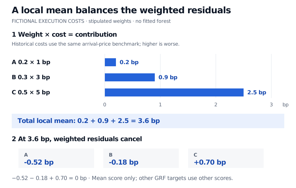
Original stipulated forest weights, not a fitted model. The mean score balances at 3.6 bp; other GRF targets require different scores.
The 3.6 bp figure is a local mean estimate under the stipulated weights, not a guaranteed cost for the target order. The three rows do not demonstrate predictive accuracy, establish a causal effect or provide a confidence interval. No forest was fitted to produce them.
Change the target, change the score
A quantile forest targets a conditional quantile, not the weighted mean. A causal forest targets a conditional average treatment effect; an instrumental-variable forest uses instrument-based moments. These are applications of the framework, not interchangeable labels. See the paper's §§5–7.
For example, estimating the effect of a new execution rule asks how costs would differ under alternative assignments. Simply predicting high costs under the rule does not answer that question. For binary treatment, the current causal-forest documentation conditions its causal interpretation on unconfounded assignment. Consistency and overlap also belong to the identification argument. Unobserved urgency affecting both rule choice and cost remains a problem.
What honesty does—and what inference still needs
Honesty assigns separate observations to choosing a tree's splits and populating its estimation leaves. Roles may differ across trees. This reduces reuse of fortunate outcome patterns in both selecting and estimating a neighbourhood. It differs from cross-fitting nuisance models. The official guide's honesty section describes this separation.
The original pointwise asymptotic theory requires iid observations, regular honest trees, suitable subsample growth, smooth identified moments and other regularity conditions—not merely many trees. See §3. In the execution example, many orders on one volatile trading day may share a shock. Randomly distributing them across leaves does not remove that dependence. An uncertainty calculation must address the sampling design; honest splitting alone does not establish valid inference for dependent financial data.
For the ensemble background, Bagging and Random Forests (membership; public preview) explains feature subsampling and aggregation.
Sources
- Athey, Tibshirani and Wager, Generalized Random Forests, Annals of Statistics 47(2), 2019. Author manuscript, April 2018 version, §§2.1–2.4, 3, 5–7.
- GRF authors, The GRF Algorithm, training, prediction and honesty. Accessed 1 November 2026.
- GRF authors, Causal forest reference, target definition and honesty arguments. Accessed 1 November 2026.