Numerical optimisation searches for the best feasible decision. A portfolio example separates the objective, bounds, global optimality and a solver’s stopping message.
Numerical optimisation
Numerical optimisation uses computational algorithms to seek a decision that minimises or maximises a specified score while satisfying the problem's restrictions. In quantitative finance, the decision might be portfolio weights, model parameters or an execution schedule. A solver can calculate a precise answer to the wrong problem, so stating the score and the allowed decisions is part of the method.
The objective function says what “better” means. A constraint says what is permitted. Their combination defines the problem, for example
A point is feasible if it satisfies every restriction. Maximising a score U(x) is equivalent to minimising f(x)=−U(x) over the same feasible set. Changing that sign changes the objective's direction; it does not remove the constraints.
A portfolio score that can be audited exactly
Consider a hypothetical one-period allocation between deterministic cash and one risky asset. Returns are simple returns in decimal units. Cash returns 0.02; the risky asset has stipulated expected return 0.08 and variance 0.04. Let w be the risky weight and 1−w the cash weight, with no borrowing or short selling:
0≤w≤1,E[Rp]=0.02+0.06w,Var(Rp)=0.04w2.
Use a mean–variance objective with risk-aversion coefficient λ=4 under these decimal-return units:
U(w)=E[Rp]−2λVar(Rp)=0.02+0.06w−0.08w2.
This score trades expected return against a variance penalty. Its numerical value is not the portfolio's expected return. The coefficient and all inputs are model assumptions, with no fees or trading costs; the result is not an investment recommendation. Changing return units requires rescaling the risk-aversion coefficient if the preference is to stay equivalent.
The derivative gives the interior candidate:
U′(w)=0.06−0.16w=0⟹w∗=83=0.375.
It is feasible. A separate calculation establishes more than stationarity:
U(w)=321−0.08(w−83)2.
The subtracted square is nonnegative for every feasible weight, so w∗ is the unique global maximiser. It gives 37.5% risky exposure and 62.5% cash, expected return 0.0425 (4.25%), variance 0.005625 and score 1/32=0.03125.
Risky weight w
Score U(w)
0
0.02000
0.25
0.03000
0.375
0.03125
0.50
0.03000
1
0.00000
The formula makes this small problem analytically soluble. That is useful: it provides an exact benchmark for checking a numerical solver before trusting a larger implementation.
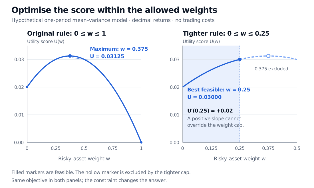
Synthetic utility U(w)=0.02+0.06w−0.08w squared. With 0≤w≤1, the maximum is w=0.375 and U=0.03125. Tightening the cap to w≤0.25 gives a boundary maximum U=0.03000 although U′(0.25)=0.02. The original maximiser is then infeasible.
Original hypothetical model. Left: the original feasible interval includes the stationary maximum. Right: tightening the cap excludes it, so the best feasible point moves to the boundary. Utility scores use decimal-return inputs; they are not realised returns.
Now change the rule to 0≤w≤0.25, keeping the objective fixed. The former maximiser is infeasible. Since U′(w)>0 throughout this smaller interval, its unique optimum is w=0.25, with U=0.03. The derivative there is still +0.02: increasing risk exposure would improve the score, but the constraint forbids it. A constrained optimum need not have zero objective gradient.
The Constrained and Convex Optimisation lesson develops active bounds and portfolio optimality conditions. Its public page is a preview; the full lesson requires membership.
What the search establishes
A local minimum has no better feasible points in a sufficiently small neighbourhood. A global minimum has no better feasible point anywhere. The distinction also applies to maximisation with the inequalities reversed.
For a convex minimisation objective over a convex feasible set, every local minimum is global. Our example has the equivalent structure: a strictly concave score maximised over an interval. A general calibration loss or a problem with discrete trade sizes need not have this structure. Running a local method from several starting points can reveal competing candidates; agreement between those runs does not prove global optimality.
An iterative method starts from a trial decision and repeatedly evaluates the objective, chooses an update and checks progress. Gradient descent uses first derivatives; Newton-type methods use curvature information; constrained methods must also handle feasibility. The objective's smoothness, available derivatives and constraint structure determine which algorithms fit.
Root finding solves an equation. Applying it to ∇f(x)=0 can find optimisation candidates, but a zero gradient alone does not distinguish a minimum, maximum or saddle. For instance, f(x)=−x2 has derivative zero at zero, which is a maximum when the task is minimisation. Boundaries also require attention, as the capped portfolio shows.
Read the stopping message with the answer
Numerical routines stop at finite precision. Depending on the method, tests may concern objective changes, step size, constraint violations or an optimality residual. A small step can reflect stagnation; exhausting an iteration budget is not an optimality certificate.
SciPy's SLSQP documentation illustrates this distinction: its precision setting enters several stopping checks, and the result separately reports success and a termination message. A tolerance is a numerical setting, not a bound on investment loss.
A useful result report includes the returned decision and objective, feasibility residuals, the stopping reason and tolerances, and the evidence supporting a local or global interpretation. Recompute the score and restrictions from the returned decision. Where available, compare with an analytic solution or a valid objective bound. In the portfolio example, the completed square supplies that global check independently of any solver's success flag.
Sources
Cornuéjols, G., Peña, J. and Tütüncü, R. Optimization Methods in Finance, 2nd ed., Cambridge University Press, 2018, Chapter 20, §§20.1–20.4, pp. 305–311: formulation, local optimality conditions and numerical algorithms.
Boyd, S. and Vandenberghe, L. Convex Optimization, Cambridge University Press, 2004, §§4.2.2–4.2.3 and 9.2: global optimality for convex problems and iterative descent methods.
SciPy development team. SLSQP minimisation documentation: precision settings, stopping criteria and returned termination information.