Multinomial distribution: Definition & Examples

The multinomial distribution gives the joint probabilities of the counts in several categories after a fixed number of independent, identically distributed trials. Each trial belongs to exactly one category. It extends the binomial distribution from a success/failure count to an entire count vector.

For a trading desk, the question might be: among the next ten orders, how many finish filled, cancelled or rejected? A multinomial model can describe that split under explicit assumptions. The individual order outcomes can be independent while the three final counts are dependent: they must share the same total of ten.

From a sequence of orders to a count vector

Let there be $k$ mutually exclusive, exhaustive categories, with fixed probabilities $p_1,\ldots,p_k$ satisfying $p_i\geq0$ and $\sum_i p_i=1$ . After $n$ independent trials, let $N_i$ count category $i$ . Write

(N_1,\ldots,N_k)\sim\operatorname{Multinomial}(n;p_1,\ldots,p_k).

The possible count vectors have nonnegative integer entries and satisfy

\sum_i N_i=n

. Their probability mass function is

\mathbb{P}(N_1=n_1,\ldots,N_k=n_k) =\frac{n!}{n_1!\cdots n_k!}\prod_{i=1}^k p_i^{n_i}, \qquad \sum_i n_i=n.

Other count vectors have probability zero. In this formula a category with zero count contributes a factor of one; if $p_i=0$ , any positive count in that category is impossible. With $n=0$ , the all-zero vector occurs with probability one.

The factorial ratio is the multinomial coefficient. Every particular ordered sequence with those counts has probability

\prod_i p_i^{n_i}

. The coefficient counts how many such sequences lead to the same vector. Rice develops this distinction in §3.2, Example A; Chen's University of Washington lecture gives the corresponding joint law and its binomial marginals.

A synthetic ten-order batch

Suppose each of ten hypothetical orders independently receives one final label:

Final category	Probability per order	Expected count in the batch
Fill	0.6	6
Cancel	0.3	3
Reject	0.1	1

These are stipulated probabilities for teaching, not estimated execution rates. The labels must partition the orders: an order with a partial fill followed by cancellation needs one agreed classification rule, rather than appearing in both counts. If pending orders remain at the observation cutoff, the three labels are not exhaustive unless the sample definition excludes them or supplies another category.

The probability of exactly six fills, three cancels and one reject is

\begin{aligned} \mathbb{P}(N_f=6,N_c=3,N_r=1) &=\frac{10!}{6!3!1!}(0.6)^6(0.3)^3(0.1)\\ &=840\times0.0001259712\\ &=0.105815808\approx10.5816\%. \end{aligned}

One particular sequence—six fills followed by three cancels and then a reject—has only the probability $0.0001259712$ . There are $\binom{10}{6}\binom{4}{3}=840$ sequences with the required counts. Omitting that multiplier answers a different question about the order of the outcomes.

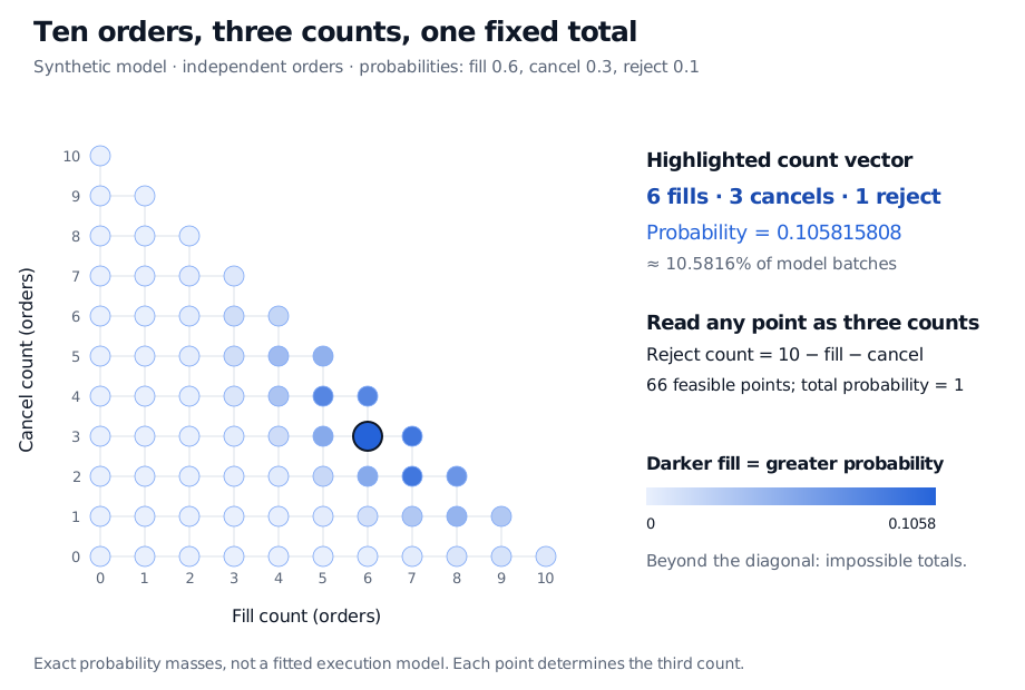
All 66 feasible count vectors for ten independent synthetic orders with fill, cancel and reject probabilities 0.6, 0.3 and 0.1. Horizontal axis is fill count and vertical axis is cancel count; reject count is ten minus their sum. Darker filled points have greater probability. The highlighted vector six fills, three cancels and one reject has probability 0.105815808.

Original exact model probabilities. Every point fixes the third count through $N_r=10-N_f-N_c$ ; points beyond the diagonal are impossible. Shading represents probability mass, not a continuous density.

Independent trials, dependent counts

Focus on one category and combine all others into “not this category.” Its marginal distribution is binomial:

N_i\sim\operatorname{Binomial}(n,p_i),\qquad \mathbb{E}[N_i]=np_i,\qquad \text{Var}(N_i)=np_i(1-p_i).

This does not make the category counts independent binomials. For two different categories,

\text{Cov}(N_i,N_j)=-np_ip_j,\qquad i\ne j.

An indicator derivation shows why. Within a trial, “fill” and “cancel” cannot both occur, so the product of their indicators is zero. Their covariance is therefore

0-p_fp_c

. Indicators from different trials have zero covariance by the independence assumption; summing over

n

trials gives

-np_fp_c

For the ten-order model, the covariance matrix, ordered fill/cancel/reject, is

\Sigma= \begin{pmatrix} 2.4&-1.8&-0.6\\ -1.8&2.1&-0.3\\ -0.6&-0.3&0.9 \end{pmatrix} \quad\text{orders}^2.

The means are $(6,3,1)$ orders; the variances are $(2.4,2.1,0.9)$ orders squared. In particular, fill/cancel covariance is $-1.8$ orders squared. This negative association follows from the model's fixed-total category allocation; it is not evidence that one operational process causally suppresses another.

Every row of

\Sigma

sums to zero. Consequently

\Sigma(1,1,1)^{\mathsf T}=0

and the matrix is singular: the sum of the three counts has variance zero. Only two counts can vary freely. An analysis that tries to invert the full matrix without accounting for this constraint has a mathematical problem even when every category has positive probability.

Combining categories also works cleanly. The number of non-fills is $N_c+N_r\sim\operatorname{Binomial}(10,0.4)$ . If only the total non-fill count matters, this collapsed model is enough; if rejects and cancels carry different costs or operational meanings, retain the joint vector.

When the model is a useful baseline

The same construction describes counts in predetermined return bins, credit-rating categories or order-status classes, provided the trials and category probabilities meet the assumptions. A single category label follows a categorical distribution; the multinomial describes the counts accumulated over repeated labels. It does not by itself model P&L amounts, order timing or the order in which events arrive.

Real orders may share a liquidity shock, have different sizes and venues, or change outcome probabilities as the book evolves. Those features can violate independence, identical probabilities, or both. Counts that sum to ten do not automatically have a multinomial law. Likewise, the displayed

(6,3,1)

are expected counts, not a guaranteed batch composition; observing those counts once would not establish that the true probabilities equal

(0.6,0.3,0.1)

For further study, Counting and Combinatorics derives the multinomial coefficient by sequential group selection (membership; public preview). Expectation, Variance and Covariance explains the moments used above (free with a signed-in account; public preview).

Sources

Rice, J. A. (2007). Mathematical Statistics and Data Analysis, 3rd ed., Duxbury. §3.2, Example A, “Multinomial Distribution”: joint mass function, binomial marginals and histogram counts.
Chen, Y.-C. (2022). STAT 512, Lecture 7: Multinomial distribution, University of Washington. Count-vector construction, marginals, category merging and covariance.

From a sequence of orders to a count vector

A synthetic ten-order batch

Independent trials, dependent counts

When the model is a useful baseline

Sources

Related terms

Binomial distribution

Independence

Indicator function

Marginal distribution

Probability mass function