The Modigliani–Modigliani measure, usually called M-squared or , expresses a portfolio's performance as a return after scaling its volatility to a chosen benchmark's volatility. It translates a Sharpe ratio comparison into familiar return units: a fund earning more than its benchmark may lose that advantage once both are compared at the same risk level.
Two reporting conventions need separating. The return level is the mean return of the hypothetical risk-matched portfolio. The benchmark-relative gap subtracts the benchmark's mean return from that level. Both are called M-squared in practice, so a reported number needs its formula and units.
Build the comparison with cash
Let be the portfolio's arithmetic expected return, its return standard deviation, and the benchmark's standard deviation. All describe the same holding period and currency. Assume a cash asset earns a certain return over that period, with no trading costs or allocation constraints.
Allocate the fraction
to the portfolio and to cash. Its simple return is , so
Cash dilutes a portfolio whose volatility exceeds the target. A portfolio below the target requires leverage: means borrowing the fraction and investing more than the initial capital in the portfolio. Liano's primary derivation develops both cases and relates the return-level formula to Modigliani and Modigliani's 1997 method.
For benchmark mean , the relative version is
where and . With one positive benchmark volatility and a common cash rate, M-squared ranks portfolios exactly as Sharpe does. It changes the presentation, not the information in that ranking.
A 10% portfolio can tie an 8% benchmark
Consider these fictional population moments of one-year simple returns. The means are arithmetic expectations; no monthly-to-annual conversion is being assumed.
| One-year quantity | Portfolio | Benchmark | Cash |
|---|---|---|---|
| Expected total return | 10% | 8% | 2% |
| Return standard deviation | 20% | 15% | 0% |
The portfolio's raw mean advantage is 2 percentage points. Its volatility is also higher. To match the benchmark, allocate to the portfolio and to cash:
The M-squared return level is 8%. The benchmark-relative gap is 0 percentage points, because . Reporting “M-squared is zero” without specifying the gap convention could wrongly suggest that the risk-matched portfolio has no expected return.
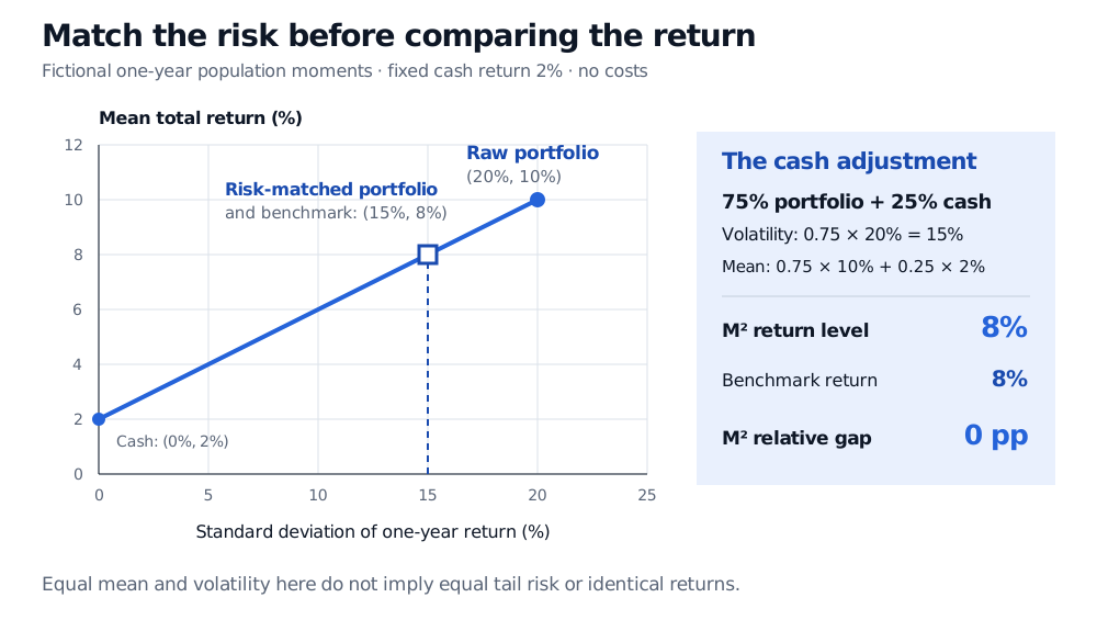
Original fictional population comparison. The line shows fixed allocations between the portfolio and riskless cash. The overlapping point matches the benchmark's mean and volatility, not its individual outcomes.
Both Sharpe ratios are : . Their equality explains the zero relative gap. Neither calculation guarantees a realised 8% return or describes compound annual growth rate.
What the adjustment leaves unresolved
Financing can change the comparison. The ideal formula uses the same risk-free rate for lending and borrowing. If and borrowing costs , the levered mean becomes . It falls below the ideal level by before other costs. Margin limits may prevent the target allocation altogether.
Historical inputs are estimates. Use aligned dates, a common frequency and a consistent fee basis for both portfolios. If cash returns vary across observations, compute cash excess returns observation by observation and explicitly state whether the target volatility concerns raw or excess returns; their standard deviations no longer have to coincide. Mixing a geometric growth rate with an arithmetic mean, or daily volatility with annual mean return, breaks the stated comparison. Sharpe's original methods discussion distinguishes historical from expected performance and explains the additional assumptions behind annualisation. Sampling error and changing volatility can make a historical risk-matched ranking unstable.
Matching volatility does not match every risk. Equal standard deviations can conceal different crash exposure, liquidity and drawdowns. Scaling a short-option strategy does not remove its rare-loss exposure. M-squared also does not match beta, hedge the benchmark, or establish manager skill: correlations and factor exposures remain relevant. A zero M-squared gap therefore means equal performance under this mean–volatility comparison, not identical investments.
For a broader comparison with beta-based and benchmark-relative measures, see Risk-Adjusted Performance Measures (public preview; the full lesson requires membership).
Sources
- Kartono Liano, A Simple Approach to Risk-Adjusted Performance (2000), Introduction and Results, equations (1)–(4): an author-hosted derivation of the risk-adjusted return level for portfolios above and below benchmark volatility.
- William F. Sharpe, The Sharpe Ratio (1994), “The Ratio,” “Time Dependence,” “Correlations” and “Scale Independence”: return-differential conventions, scaling assumptions and the limits of mean–variance comparisons.