Add a square matrix’s diagonal entries, use cyclic trace rules correctly, and distinguish covariance trace from a portfolio’s variance and PCA retention.
Matrix trace
The trace of a square matrix is the sum of its main diagonal entries. For an n×n matrix A,
tr(A)=i=1∑naii.
The main diagonal runs from the top left to the bottom right. Trace returns one number, not a vector or a matrix. The standard definition requires a square matrix; summing the available diagonal entries of a rectangular array is not the trace operation used here.
For a covariance matrix, the diagonal contains individual variances. Its trace therefore measures their sum. This is useful when compressing a return model into principal components—but it does not give the variance of a particular portfolio.
A risk report with three different answers
Suppose a risk team stipulates this synthetic covariance matrix for two assets’ one-year simple returns, expressed as decimals:
Σ=(0.040.010.010.09).
The asset return standard deviations are 20% and 30%. Each diagonal entry is a variance in decimal-return squared over the stated one-year horizon. The trace is
tr(Σ)=0.04+0.09=0.13.
This sums dispersion across the two asset coordinates. It does not specify how much money is invested in either asset. In particular, 0.13 is neither a 13% volatility nor a portfolio variance awaiting only a square root.
For a fully invested 50/50 portfolio held over that same period, the return is Rp=0.5R1+0.5R2. Its portfolio variance includes the covariance:
The portfolio’s one-year standard deviation is 0.0375≈19.36%. Changing its weights or the off-diagonal covariance changes this risk even when the trace stays fixed. Trace cannot report diversification by itself.
A third question asks how much of the two-coordinate variation a one-component principal component analysis retains. The covariance eigenvalues are approximately
λ1=0.091925824,λ2=0.038074176.
They sum to 0.13. The leading component retains
tr(Σ)λ1=0.130.091925824≈70.7%.
That is the fraction of aggregate coordinate variance retained by this PCA approximation. It is not a promise to retain 70.7% of every portfolio’s risk: a portfolio pointing entirely along the discarded component would lose all its modelled variance in a one-component approximation. Nor is variance retention a forecast-accuracy or tail-risk guarantee. The covariance-trace interpretation and retention ratio are developed in Penn State’s PCA notes.
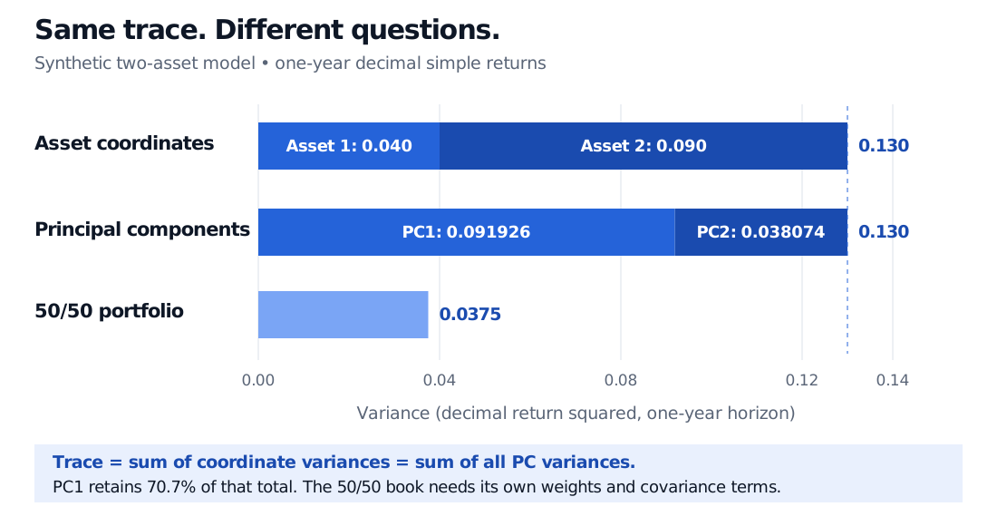
Synthetic one-year decimal-return covariance: asset variances 0.040 and 0.090 sum to trace 0.130. Principal-component variances 0.091926 and 0.038074 also sum to 0.130; PC1 retains 70.7%. The separate 50/50 portfolio has variance 0.0375.
Original synthetic covariance example. Both stacked bars decompose the same trace; the single portfolio bar answers a different question. All horizontal values are one-year decimal-return variances, not volatilities.
The rule that moves a product around a trace
Trace is linear: for same-sized square matrices and scalars α,β,
tr(αA+βB)=αtr(A)+βtr(B).
Its most useful product rule is cyclic. If A is m×n and B is n×m, then AB is m×m, BA is n×n, and
tr(AB)=i=1∑mj=1∑naijbji=tr(BA).
Both sides sum the same scalar products. The matrices themselves can have different sizes and need not be equal. MIT’s matrix-algebra notes, Result 22, collect these trace identities.
For three factors with shapes A:m×n, B:n×p, C:p×m,
tr(ABC)=tr(BCA)=tr(CAB).
Move the first factor to the end while preserving cyclic order. Arbitrarily swapping two factors is not valid: even when every product exists, tr(ABC) need not equal tr(ACB).
This also gives a useful bridge back to portfolio risk:
w⊤Σw=tr(Σww⊤).
The left side is a scalar, equivalently a 1×1 matrix. On the right, the weights appear through ww⊤. They have not vanished; replacing this expression with tr(Σ) would discard them.
What survives a change of coordinates?
If P is invertible, the change of basis for a linear operator gives a similar matrix P−1AP. Cyclicity proves
tr(P−1AP)=tr(APP−1)=tr(A).
Trace also equals the sum of all eigenvalues, counted with algebraic multiplicity, allowing complex eigenvalues. Diagonalisation is not required. See Quinlan’s §1.2 for similarity and the general eigenvalue connection. The determinant multiplies eigenvalues; trace adds them. A zero trace does not imply singularity: the invertible diagonal matrix with entries 1 and −1 has trace zero. For a covariance matrix, positive semidefiniteness makes all eigenvalues nonnegative; a general square matrix has no such restriction.
There is a subtle distinction for random-vector coordinates. If returns are transformed as Y=LR, their covariance becomes LΣL⊤, not generally LΣL−1. When L is orthogonal, L⊤=L−1, so trace is preserved. PCA uses precisely such an orthogonal rotation. An arbitrary rescaling need not preserve it: doubling only the first asset’s return coordinate changes the example’s diagonal variances to 0.16 and 0.09, giving trace 0.25.
Units matter too. Converting both returns from decimals to percentage points multiplies every covariance by 1002, so trace becomes 1,300 percentage-points squared. Standardising each nonconstant asset to unit variance instead gives a correlation matrix, whose trace is simply the number of assets—two here—regardless of their correlation. Both operations change the variance scale being summarised; neither is a reduction in economic risk.