The Lilliefors test is a goodness-of-fit test that uses the largest gap between an empirical CDF and a fitted distribution, with calibration that accounts for estimating parameters from the tested sample. Its best-known version asks whether independent observations could come from a normal distribution with an unknown mean and variance. For a quant checking return-model assumptions, the crucial point is that fitting the mean and volatility changes the reference distribution of the test statistic.
The curve has already seen the data
An ordinary one-sample Kolmogorov–Smirnov test compares observations with a continuous distribution specified in advance. A normality check usually estimates the normal curve from those very observations. The fitted curve adapts to the sample, so the ordinary fixed-CDF KS calibration no longer applies. R's official
ks.test documentation explicitly excludes estimating the reference parameters from the tested data. R documentationLilliefors keeps the maximum-gap idea and changes its calibration. This is a composite null: some mean and some positive variance within the normal family may have generated the data. Rejecting it challenges that family; failing to reject does not establish normality. CRAN nortest manual
Compute the distance, then calibrate it
For sorted observations , define the fitted normal CDF by
Here is the standard normal CDF and uses the sample variance divisor . Both sides of each empirical-CDF jump matter:
This article uses the unscaled distance , without a multiplier. The formulas follow the normality version in the nortest manual; statsmodels likewise standardises with divisor . A fitting rule, statistic convention and critical-value calibration must match. Replacing with a divisor- estimate without checking the calibration changes the procedure. Statsmodels implementation
Take five fictional observations in arbitrary units, sorted as . They give and .
| Fitted normal CDF | ||||
|---|---|---|---|---|
| 1 | −1 | 0.12587 | 0.07413 | 0.12587 |
| 2 | 0 | 0.31848 | 0.08152 | 0.11848 |
| 3 | 0.5 | 0.44637 | 0.15363 | 0.04637 |
| 4 | 1 | 0.58014 | 0.21986 | −0.01986 |
| 5 | 3 | 0.93951 | 0.06049 | 0.13951 |
Thus , and . The largest gap occurs at , where the empirical CDF has jumped to .
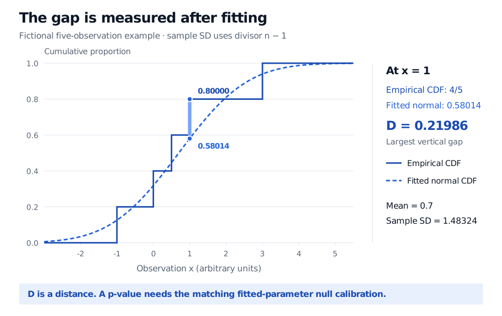
Original fictional example. The highlighted vertical distance is the unscaled statistic D; it is not a p-value or a rejection threshold.
The table establishes the statistic only. It supplies neither a significance result nor persuasive evidence of normality from five observations.
What a usable result needs
A valid p-value needs a null distribution calibrated for this fitting procedure and sample size. Statsmodels provides separate normal and exponential versions, with simulation-based tables. The exponential version estimates its mean with the origin fixed at zero; it is not a normality test, and its calibration is not interchangeable with the normal version. Statsmodels API, implementation
For a simulation calibration, each replicate must repeat the fitting step before computing its distance. Holding the original fitted parameters fixed in every replicate recreates the wrong testing problem. A parametric bootstrap can implement this fit-and-test workflow, subject to the model and estimator used. SciPy goodness-of-fit documentation
For financial data, check the sampling story too. Standard iid continuous-sample calibration does not automatically cover serial dependence, volatility clustering, or residuals created by fitting a time-series model. Such residuals can inherit estimation constraints and dependence; any simulation needs to reproduce the relevant model-fitting pipeline. R also warns that ties and rounding affect one-sample KS calculations. A fitted-normal p-value cannot repair those sampling mismatches. R documentation
To understand the curve comparison, read The Empirical CDF, Glivenko–Cantelli, and QQ-Plots. Its public preview introduces the lesson; the full teaching requires membership. A QQ-plot helps locate a shape mismatch that a single maximum distance compresses into one number.