Goodness of fit: Definition & Examples

Goodness of fit describes how closely a statistical model agrees with observed data, judged by a chosen discrepancy. A goodness-of-fit test asks whether a discrepancy at least as large as the observed one would be unusual under the model and its sampling assumptions.

An execution model may predict the proportions of fully filled, partly filled and unfilled orders. A return model may predict the whole distribution of daily profit and loss. Both can fit one feature while missing another: matching the mean does not establish the right loss tail, and matching outcome proportions does not establish independent outcomes.

Specify what “fits” means

A fit assessment needs a target, a discrepancy and a reference for how much random variation to expect. These choices determine what the assessment can detect.

Assessment	What it compares	What to watch
Pearson’s categorical test	Observed category counts versus model expected counts	Binning can hide departures within categories; the usual chi-squared reference is approximate.
Kolmogorov–Smirnov test	The largest gap between an empirical and reference cumulative distribution	The standard continuous one-sample calibration requires a fully specified reference distribution.
Quantile–quantile plot	Observed quantiles versus model quantiles	Shows where shape departs, but a visual deviation alone has no calibrated rejection probability.

These assessments complement one another. A plot can reveal which tail is wrong after a test flags a discrepancy. A single reported fit score cannot describe every way a model might fail.

A model that is not rejected

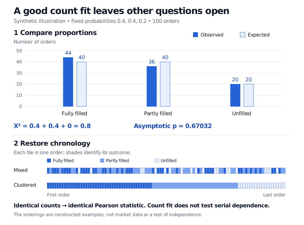
Suppose a hypothetical execution model assigns fixed probabilities $0.4$ , $0.4$ and $0.2$ to fully filled, partly filled and unfilled orders. The categories are exhaustive and mutually exclusive. We stipulate $100$ independent orders with the same probabilities; neither the categories nor the probabilities were selected using these observations.

The resulting counts have a multinomial distribution under the model. Observed and expected counts are:

Outcome	Observed $O_i$	Expected $E_i$	Contribution $(O_i-E_i)^2/E_i$
Fully filled	44	40	0.4
Partly filled	36	40	0.4
Unfilled	20	20	0

Pearson’s statistic adds squared deviations, scaled by expected counts:

X^2=\sum_{i=1}^{K}\frac{(O_i-E_i)^2}{E_i}, \qquad E_i=np_i.

Here $K$ is the number of categories, $n$ is the total number of orders, and $p_i$ is the fixed null probability for category $i$ . Thus

X^2=\frac{4^2}{40}+\frac{(-4)^2}{40}+\frac{0^2}{20}=0.8.

With three categories and no estimated parameters, the large-sample reference is a chi-squared distribution with

K-1=2

degrees of freedom. All expected counts here are at least

20

; sparse cells are not the concern in this example. The reference remains an approximation to the finite count experiment.

The upper-tail p-value is approximately

p=\mathbb{P}(\chi^2_2\ge0.8)=e^{-0.4}\approx0.67032.

At a prespecified

5\%

significance level, we do not reject the stated probabilities. This result says the chosen count discrepancy is unremarkable under that model. It does not give a 67% probability that the model is correct. Nor does nonrejection prove a sufficiently accurate model for an execution decision: the test may have limited power against a commercially important departure.

Observed counts 44, 36, 20 versus expected counts 40, 40, 20 give Pearson statistic 0.8 and asymptotic p approximately 0.67032. Mixed and clustered order sequences preserve those same counts, so the statistic cannot distinguish them.

Figure: Original synthetic example. The same outcome counts can conceal very different chronology; the figure’s orderings are constructed illustrations.

The lower panel exposes a limit of this particular comparison. Rearranging the outcomes leaves the statistic unchanged, although a clustered history would raise a separate question about independence. A count test alone cannot validate a model’s serial structure. Actual order outcomes can share market conditions or parent orders, making the independent-order assumption inappropriate.

Fit after fitting needs its own calibration

If model parameters are estimated from the same observations, the model has already adjusted toward the sample. A reference law for a fixed model cannot automatically be reused. Pearson’s familiar degrees-of-freedom adjustment needs the appropriate grouped-data fitting and regularity conditions. Standard continuous Kolmogorov–Smirnov tables likewise need adjustment when the reference parameters were fitted from the tested sample.

For the derivation and the grouped-versus-ungrouped fitting distinction, see Goodness-of-Fit Tests (public preview; full lesson requires membership).

For model validation, report what was compared, how parameters were obtained, the sampling assumptions, and the size and location of departures. Then ask whether those departures affect the intended decision. Goodness of fit supplies evidence about a model at a stated resolution; it cannot certify future market behaviour.

Sources

John A. Rice, Mathematical Statistics and Data Analysis, 3rd edition, Duxbury, 2007, §§9.2.1, 9.5 and 9.9: p-value interpretation, multinomial goodness of fit and parameter-estimation caveats.
NIST/SEMATECH, “Chi-Square Goodness-of-Fit Test”: count statistic, binning and approximate calibration.
NIST/SEMATECH, “Kolmogorov–Smirnov Goodness-of-Fit Test”: empirical-distribution comparison and fitted-parameter limitation.
R statistical documentation, “Pearson’s Chi-squared Test for Count Data”: fixed categorical probabilities and asymptotic versus simulated p-values.

Specify what “fits” means

A model that is not rejected

Fit after fitting needs its own calibration

Sources

Related terms

Chi-squared distribution

Independence

Multinomial distribution

P-value