An equity-index future and a constituent stock are a possible research pair: price discovery may happen at different speeds. That is a hypothesis about information transmission, not a promise that every futures move predicts the stock. Unlike a conventional pairs trade, the signal need not be a price spread expected to revert. The central feature is a directional, time-ordered relationship.
What exactly leads?
Here indexes interval endpoints and positive means A’s return comes earlier. A relationship can be positive or negative; “leader” names the temporal ordering, not the sign. Comparing positive and negative lags helps distinguish A-leading-B from the reverse ordering. The interval length and price definition must be stated: a five-minute last-trade return answers a different question from a sequence of quote changes.
A correlation peak is a diagnostic, not yet a forecast that improves on B’s own history. Test whether A adds information beyond the chosen baseline and shared market drivers. A common announcement can reach both markets while producing different adjustment speeds; this does not establish that trading in A causes B to move.
Scenario 1: the event is early; the message is late
| Event | Time |
|---|---|
| A’s market event occurs | 0.100 |
| A historical replay submits a response using that event | 0.150 |
| B’s market price moves | 0.200 |
| A’s message reaches this strategy locally | 0.250 |
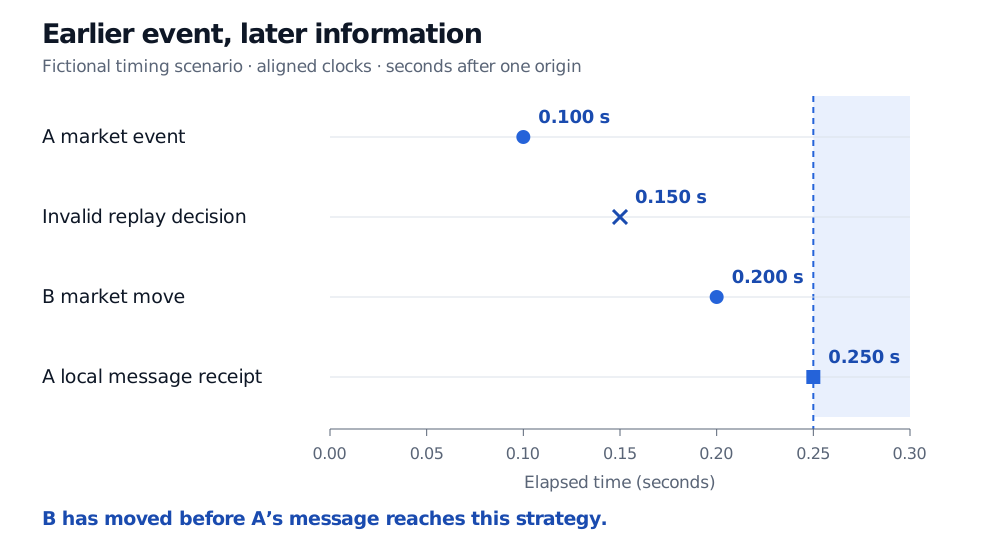
Original fictional timing scenario, with exact aligned clocks for illustration. The shaded interval begins at local receipt; processing and order-routing delays would push feasible action later still.
The illustration assumes perfect clock alignment only to isolate the receipt problem. In real cross-market data, timestamp resolution and clock-offset uncertainty can be comparable to the measured lag. If the uncertainty intervals do not establish an ordering, report it as unresolved. A precisely printed timestamp is not evidence of an equally accurate clock.
Scenario 2: a forecast is timely, but the midpoint is not a fill
Evidence that survives a replay
A useful research design must challenge both the measured relationship and the trading policy:
- Audit the observations. Check timestamp meanings, sequence gaps, stale quotes, corrections and overlapping trading hours. Compare trade-price and quote-based results: bid-ask bounce can contaminate trade returns even without a change in underlying value.
- Preserve the information boundary. Replay receipt order and processing delays; start the forecast’s tradeable outcome after feasible entry. A future endpoint alone does not make a return interval eligible if part of it occurred before entry.
- Freeze the research choices. Choose assets, lag windows and thresholds on training data, then evaluate in later periods. Trying many pairs and keeping the strongest peak invites overfitting. Check stability across sessions and news conditions rather than treating one fitted lag as permanent.
- Reconcile positions with fills. Model entry and exit liquidity, fees, transaction costs, inventory exposure and any hedge. A follower-only position remains exposed to its own news; a cross-market hedge adds basis, funding and execution risks. Passive orders need a fill model, not an assumption of free spread capture.
Lead-lag evidence becomes economically useful only when information arrives early enough, prediction persists outside the fitting sample, and feasible trades retain value after costs. Temporal association by itself establishes none of those conditions.
Sources
- Huth and Abergel, High Frequency Lead/lag Relationships — Empirical facts, author preprint: §2.1 on asynchronous observations and lagged correlation; §§3.5–3.6 on quote responses and the distinction between forecasting and spread-adjusted trading results. Historical research, not current market calibration.
- Hoffmann, Rosenbaum and Yoshida, Estimation of the lead-lag parameter from non-synchronous data, Bernoulli 19(2), 2013: §1.1 on the estimation problem and its limits; §2.1 on the time-shift model. The two scenarios above are original teaching constructions.