Layer normalisation standardises hidden features within an example. See the token-wise axes, positive epsilon and learned affine step, and why none guarantees a causal financial forecast.
Layer normalisation
Layer normalisation standardises a group of hidden activations within one example, then usually applies a learned scale and shift. In a sequence model processing financial text or market observations, a common choice is to normalise the hidden features of each token separately. Its statistics do not depend on which other examples share the batch, making it useful when long sequences constrain batch size.
The decisive question is which entries supply the mean and variance? “Normalise the layer” is too vague to answer it.
One token is one statistic group
Suppose a hidden-state tensor has axes batch, token and feature. For token-wise layer normalisation, fix the batch item and token, and aggregate only over its d hidden features. Write those values as x1,…,xd:
Here v is the population-style variance over this group, with divisor d, rather than an unbiased estimator with divisor d−1. The positive constant ε prevents division by zero. The gain γ and bias β are learned parameters, not fresh estimates from each token.
Ba, Kiros and Hinton’s original paper defines within-example statistics in §3 and applies them separately at each recurrent time step in §3.1. Layer normalisation uses current-input statistics at both training and inference; it needs no running batch averages.
The axes are a design choice. In Keras LayerNormalization, axis=-1 selects the final dimension, and the learned parameters span the selected axes. Other implementations can choose different parameter-sharing axes. Match both the reduction axes and the parameter shapes when reproducing a model.
Standardisation is only the first step
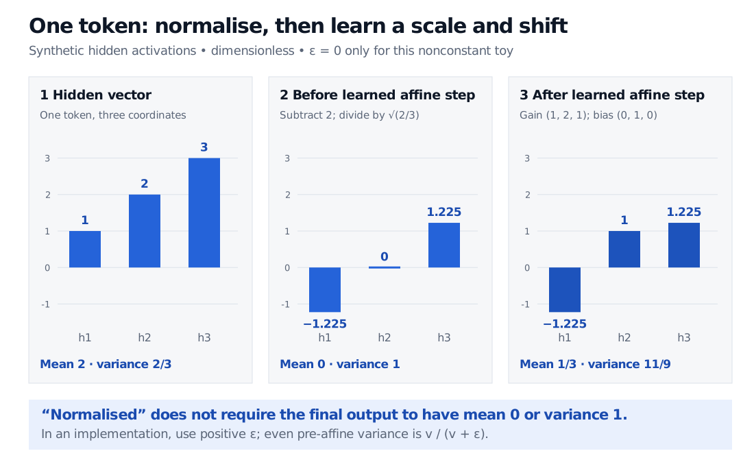
Take one synthetic token whose three hidden coordinates are (1,2,3). They are dimensionless activations, not three raw financial quantities with different units. Their mean is 2, and their population variance is 2/3.
For this nonzero-variance arithmetic illustration only, set ε=0. Standardisation gives
z=(−23,0,23).
Now choose illustrative learned gains (1,2,1) and biases (0,1,0). The middle normalised coordinate is zero, so its gain has no effect here; its bias moves it to one:
y=(−23,1,23).
The final output has mean 1/3 and population variance 11/9. Thus “layer-normalised” does not mean every final output must have mean zero and variance one.
Three stages for one synthetic token: hidden coordinates 1, 2, 3; pre-affine coordinates approximately minus 1.225, 0, plus 1.225; affine output approximately minus 1.225, 1, plus 1.225. The epsilon-zero toy has pre-affine mean zero and variance one, but final mean one third and variance eleven ninths.
Original synthetic hidden-vector calculation; all values are dimensionless. Epsilon is zero only to expose the arithmetic for a nonconstant vector. Implementations use positive epsilon; the learned affine step need not preserve mean or variance.
With positive epsilon, even the pre-affine vector has variance v/(v+ε), rather than exactly one; its mean is zero in exact arithmetic. If all coordinates are equal, the centred vector is zero, and the affine output is simply the bias vector. Epsilon belongs in a real implementation even though the toy calculation above omits it.
INTERACTIVE EXPLORER
Normalisation reduction axes
Compare row, column, group and RMS statistics on a small tensor.
Similar names, different reductions
On a two-dimensional table with examples as rows and features as columns:
One row’s uncentered mean square; no mean subtraction
The table deliberately excludes spatial dimensions. Image architectures can include spatial positions in their statistic groups; inspect the actual tensor layout rather than transferring this table unchanged. Keras’s group-normalisation documentation describes channel grouping, while its layer-normalisation page cautions that matching normalisation groups alone need not match learned parameter shapes. RMS normalisation is distinct because it rescales without centring.
What this changes in a quant model
Normalising each token’s feature vector avoids pooling statistics from unrelated batch members. It does not certify the information set behind that vector. If a hidden state already includes tomorrow’s return, centring and rescaling it leaves the look-ahead bias intact. Pooling statistics over an entire time sequence can itself mix future and past positions; token-wise reduction avoids that particular mixing, but does not replace causal attention masks, point-in-time inputs or chronological validation.
Layer normalisation also operates on learned representations; it is not a substitute for choosing sensible units and fitting input preprocessing on training data. Its suitability and its placement relative to a residual network remain architecture choices, to assess through optimisation behaviour and held-out performance rather than assume from the name.