Group normalisation standardises channel groups within each example. See its calculation, spatial axes, learned parameters and the limits of batch independence.
Group normalisation
Group normalisation (GN) centres and rescales a neural network's activations within groups of channels, separately for each example. In a convolutional layer, each group also includes its spatial positions. It can be useful when a quant model's large inputs constrain batch size: a single observation's normalisation does not depend on the other observations placed in its mini-batch.
“Group” means a group of channels inside one example, not a group of securities, trading days or examples. The channels are internal features of the neural network; they need not correspond to economic sectors.
The boundary around a statistic
For an activation tensor with batch, channel, height and width axes, write its shape as (N,C,H,W). Split the C channels into G equally sized groups, with C divisible by G. For one example and one channel group, pool the (C/G)HW activation values. Their mean and variance supply the denominator for every activation in that group; another example supplies its own statistics. This is the construction in Wu and He's Group Normalization paper, §3.
Let Sn,g contain the entries in example n, group g, including all spatial positions, and let m=(C/G)HW. Then
The variance divides by the number of entries m, rather than m−1. The learned scale γc and offset βc are per channel, shared over that channel's spatial positions. They are not one pair per group. Use positive ϵ to keep the denominator defined when the group is constant.
Four channels, two local comparisons
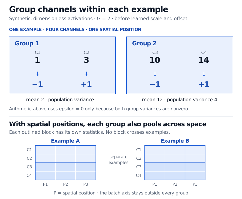
Take one fictional example with four dimensionless channel activations, at one spatial position: (1,3,10,14). Set G=2, so the groups are (1,3) and (10,14).
Group
Mean
Divide-by-count variance
Pre-affine outputs with ϵ=0
Channels 1–2
2
1
(−1,1)
Channels 3–4
12
4
(−1,1)
Here ϵ=0 is only a nonzero-variance arithmetic illustration. For example, the second group gives (10−12)/2=−1 and (14−12)/2=1. No statistic from another example enters either calculation.
One synthetic example has channel values 1, 3, 10 and 14. Two channel groups have means 2 and 12 and population variances 1 and 4, producing minus 1, plus 1, minus 1, plus 1 before affine transformation with epsilon zero. The lower diagram shows separate groups pooling two channels and three spatial positions inside each example, never across examples.
Original synthetic calculation and axis diagram. All activation values are dimensionless; epsilon is zero only in the nonzero-variance calculation above.
Pooling all four values instead gives mean 7 and variance 27.5. That changes what an activation is compared with: the high-valued second group now affects the first group's reference level. GN's grouping is therefore part of the model specification, rather than a cosmetic reshaping step.
Positive epsilon also matters mathematically: the within-group variance of x is v/(v+ϵ), not exactly one. Applying different learned channel scales and offsets changes the output moments again. A constant group centres to zero and yields the corresponding channel offsets; it does not yield infinite activations.
G=1: GN pools all channels and spatial positions of each example. This matches layer normalisation's statistics when layer normalisation is configured to reduce over those same axes. Normalising only a token's feature dimension is a different operation.
G=C: each group has one channel, so its statistics pool that channel's spatial positions, matching instance normalisation's reduction axes. In our one-position example each group is a singleton, so the mathematical pre-affine result is zero with positive epsilon. A real spatial feature map usually has multiple values per channel; one channel per group does not then imply a zero result.
These statistical identities do not guarantee interchangeable library layers. PyTorch LayerNorm can learn a separate affine pair for every element of its normalised shape, whereas GN shares its pair across each channel's positions. InstanceNorm2d defaults to no learned affine transform and can optionally use running statistics at evaluation. Matching axes, epsilon, affine parameters and evaluation behaviour is necessary before claiming equal outputs; implementations can also reject degenerate shapes.
Batch independence has a limited meaning
PyTorch GroupNorm uses current-input statistics in both training and evaluation, rather than replacing them with running batch estimates. Holding an example's activations and the learned parameters fixed, changing its batch neighbours cannot change that GN calculation. This removes one particular source of cross-example dependence; it does not make the training algorithm independent of batch size. Mini-batches still affect gradient estimates and optimisation.
Wu and He's experiments concern image classification, detection, segmentation and video. Their small-batch results motivate testing GN in memory-constrained architectures; they do not establish better financial forecasts or trading performance. Choose the group count using the training and validation design, with the final test period held aside.
For a causal time-series model, also inspect which positions are pooled. If time is treated as a spatial axis, pooling an entire window can make an early position depend on later positions in that window. Per-example statistics do not by themselves prevent look-ahead bias. A prediction made only after the whole window is available has a different information boundary.