Residual networks add learned corrections to shortcuts. Trace a scalar block and its gradient, understand projection and activation order, and avoid guarantees about financial generalisation.
Residual network
A residual network is a neural network built from blocks that add a learned transformation to a shortcut carrying the block's input. This lets a deep model refine an existing representation instead of requiring each block to reconstruct it. For a quant researcher building a deep encoder for order-book observations or volatility surfaces, the immediate benefit is an architectural way to ease optimisation; forecasting value still has to be established on later data.
Learn a correction to the input
For an input vector or tensor x, the simplest identity-shortcut block computes
y=x+F(x;θ).
The residual branch F contains trainable layers with parameters θ. If a desired block mapping is H(x), the branch is asked to learn H(x)−x. When F(x)=0, this basic block passes x through unchanged. Here “residual” means a correction relative to the input, rather than an observed-minus-predicted regression error.
He and colleagues introduced the ResNet family to address degradation: deeper plain networks could have higher training error than shallower counterparts. That is an optimisation problem, distinct from overfitting. Their 2015 paper, §§1 and 3, motivates the residual parameterisation and tests it on image-recognition tasks.
The addition is element by element. Both branches must have matching shapes; concatenation would append features and is a different operation. When channels or resolution change, a common repair is a learned projection shortcut:
y=P(x)+F(x;θ).
In a convolutional neural network, this can be a 1×1 convolution with an appropriate stride and output-channel count. The shortcut then has parameters and is no longer the identity map. See He et al., §3.2.
Follow the value, then the gradient
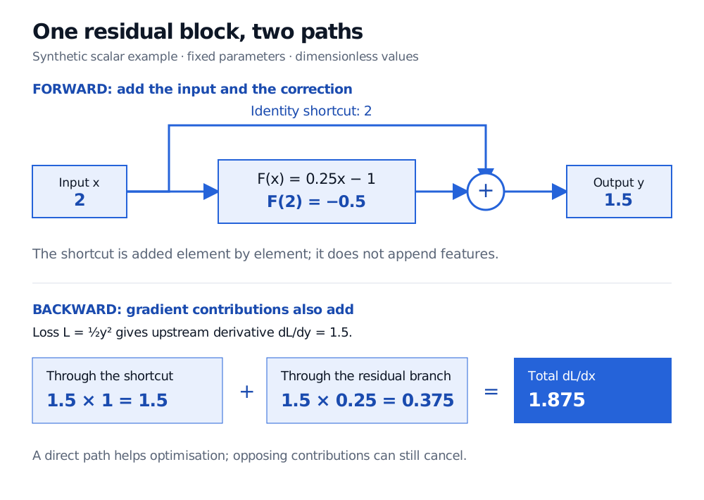
Take a synthetic, dimensionless scalar block with fixed branch F(x)=0.25x−1. At x=2, the branch produces −0.5 and the addition gives y=1.5. These values illustrate the computation; they are not fitted financial estimates.
Synthetic input 2 follows an identity shortcut and residual branch F(x) equals 0.25x minus 1, producing minus 0.5. Addition gives output 1.5. For loss half y squared, shortcut and branch gradient contributions are 1.5 and 0.375, summing to 1.875.
Original scalar forward and backward calculation. Parameters are fixed by hand; all quantities are dimensionless. The diagram shows addition before any optional output activation.
For a differentiable scalar branch, the block derivative is
The two paths contribute 1.5 and 0.375. This derivative concerns the block's input; updating a trainable parameter requires its own loss derivative. In the vector case, the block Jacobian is I+JF(x), where I is the identity matrix and JF is the branch Jacobian. The 2016 identity-mapping paper, §2, analyses the direct forward and backward paths created by identity shortcuts.
A direct path does not guarantee a nonzero total gradient. Set F(x)=−x+3: the basic block is constantly 3, so its input derivative is 1−1=0. Even with L=21y2 and nonzero upstream derivative dL/dy=3, the total dL/dx is zero. Nor does the identity summand guarantee good conditioning or prevent exploding gradients across a whole network.
The activation's position changes the block
The displayed equation describes the addition itself. The original ResNet units apply a ReLU after that addition, so a full post-activation unit outputs ReLU(x+F(x)). Negative sums are clamped to zero and their local derivatives are zero. Even F=0 then gives ReLU(x), rather than the identity for every possible input.
Full pre-activation units move normalisation and ReLU before the branch's weight layers and leave the sum without an immediate post-addition ReLU. This preserves a cleaner identity route across compatible blocks. He et al. compare these orderings in the 2016 paper, §4 and Figure 4. “Residual connection” alone therefore does not specify the activation order or the shortcut used at shape changes.
Use depth as a research choice
A residual architecture can improve trainability without demonstrating better predictions outside the training sample. There is no universal layer count at which shortcuts become necessary, and image-benchmark results do not establish an advantage on a financial dataset. Compare the complete training procedure with a simpler baseline under the same evaluation rules.
For a forecasting encoder, every residual branch still needs to respect the prediction cutoff. Adding an identity path does not repair a branch that uses future observations. Keep preprocessing, parameter fitting and architecture selection within their eligible data windows, then evaluate on later observations; shortcuts do not remove look-ahead bias or protect against distribution shift.
He, Zhang, Ren and Sun, Deep Residual Learning for Image Recognition, 2015, §§1, 3.1–3.2. Degradation, residual parameterisation, post-addition activation and projection shortcuts.
He, Zhang, Ren and Sun, Identity Mappings in Deep Residual Networks, 2016, §2 and §4, especially Figure 4. Identity-path analysis and post-activation versus pre-activation units.