Activation variants and saturation: Definition & Examples

An activation function transforms a unit's pre-activation, usually a weighted sum plus a bias, into its output. Saturation means that this output becomes insensitive to further changes in the input: its local derivative approaches zero. In a neural network processing returns, volumes or order-book features, the choice of activation and the scale reaching it affect both the representation and how readily its incoming weights can learn.

Write a scalar unit as $z=\mathbf{w}^{\top}\mathbf{x}+b$ and $a=f(z)$ . If the loss is $L$ , the chain rule gives

\frac{\partial L}{\partial z} =\frac{\partial L}{\partial a}f'(z).

The activation derivative is one factor in the gradient, alongside weights and derivatives elsewhere in the network. Repeated small factors can contribute to vanishing gradients; inspecting one activation alone does not diagnose the entire network.

Almost the same output, very different slopes

The logistic sigmoid and hyperbolic tangent are

\sigma(z)=\frac{1}{1+e^{-z}},\qquad \sigma'(z)=\sigma(z)(1-\sigma(z)),\qquad \frac{d}{dz}\tanh(z)=1-\tanh^2(z).

At a stipulated, unitless pre-activation of $z=10$ :

Activation	Output	Local derivative
Sigmoid	$0.9999546$	$4.5396\times10^{-5}$
tanh	$0.9999999959$	$8.2446\times10^{-9}$
ReLU	$10$	$1$

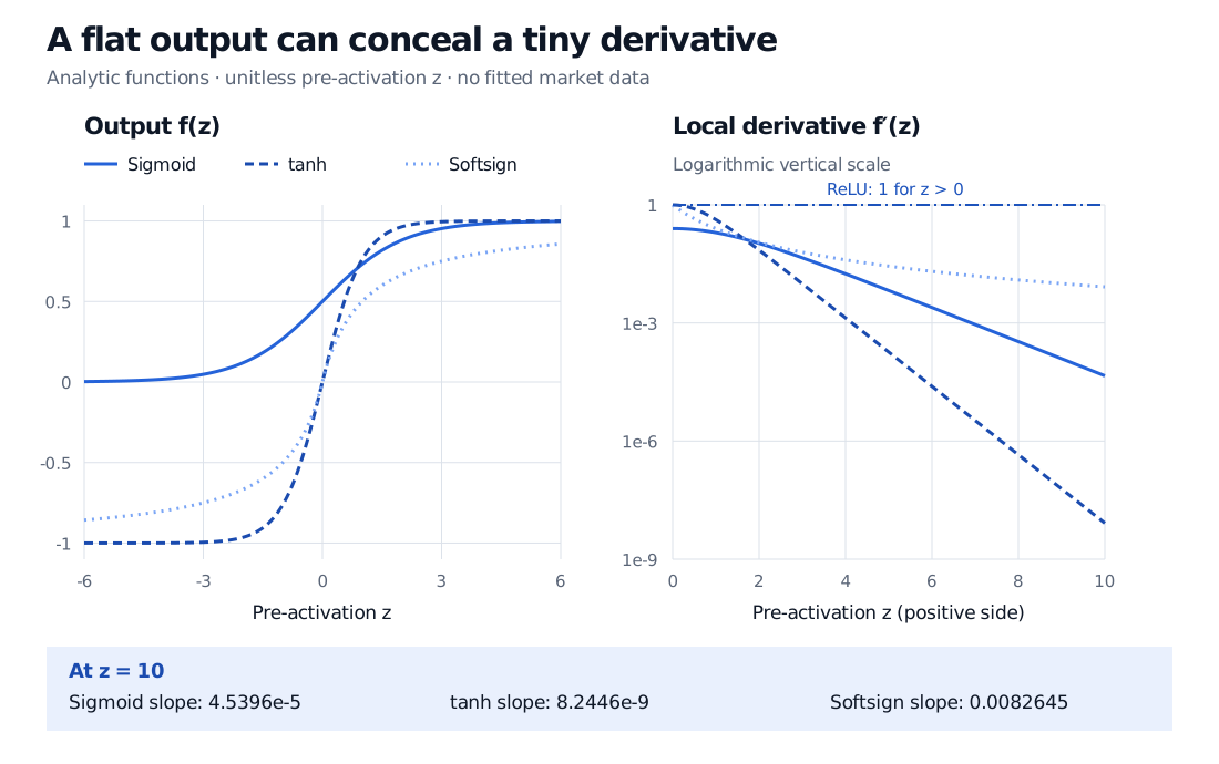
Both bounded activations are near their upper limits, but tanh has a much smaller slope at this particular input. This is not a universal ranking: at zero, tanh's derivative is one and sigmoid's is one quarter. Goodfellow, Bengio and Courville, §6.3.2, explain the hidden-unit saturation mechanism.

Analytic sigmoid, tanh and softsign output curves alongside their positive-side derivatives on a logarithmic scale. At z equals 10, sigmoid slope is 4.5396 times 10 to the minus 5, tanh slope is 8.2446 times 10 to the minus 9, softsign slope is 0.0082645, and positive ReLU slope is one.

The logarithmic derivative axis reveals differences that the bounded output curves conceal. ReLU's reference line applies only to positive inputs.

These are mathematical derivatives, rounded for display. Floating-point evaluation can lose a tiny slope when subtracting two nearly equal numbers. For example, evaluating $1-\tanh^2(z)$ at sufficiently large positive $z$ may return zero because the computed tanh has already rounded to one. The equivalent expression $4e^{-2\lvert z\rvert}/(1+e^{-2\lvert z\rvert})^2$ avoids that subtraction, although its exponential eventually underflows too.

Different remedies change different things

ReLU uses

f(z)=\max(0,z)

. Its slope is one for positive inputs and zero for negative inputs. It is not differentiable at zero; an implementation must choose a backward-pass convention there. A unit that is inactive for one observation is not necessarily a dead ReLU. Deadness describes persistent inactivity across the relevant inputs, leaving no data-loss gradient through that unit's incoming parameters. Other parameter changes can still move its inputs. This flat negative branch differs from sigmoid or tanh approaching a limiting value asymptotically.

Leaky ReLU replaces the negative branch by

\alpha z

, here with fixed

0<\alpha<1

. Negative inputs then have slope

\alpha

. PReLU learns the negative slope instead of fixing it. A nonzero slope removes ReLU's exactly flat negative branch, but a very small slope can still attenuate gradients. See He et al., §2.1.

Softsign keeps a bounded output:

f(z)=\frac{z}{1+\lvert z\rvert},\qquad f'(z)=\frac{1}{(1+\lvert z\rvert)^2}.

Its slope still approaches zero, but polynomially rather than exponentially. At ten it is

1/121\approx0.0082645

. Gentler tails modify saturation; they do not eliminate it. Glorot and Bengio, §§2–3.3, compare softsign with sigmoid and tanh.

GELU uses

f(z)=z\Phi(z)

, where

\Phi

is the standard normal cumulative distribution function. Here GELU means that exact function; the frequently used tanh expression is an approximation, not an identity. Its derivative is

\Phi(z)+z\varphi(z)

, with

\varphi

the standard normal density. Thus even a smooth activation can have slope above one: at

z=1

, GELU's derivative is approximately

1.083

. See Hendrycks and Gimpel, §2.

Swish uses

f(z)=z\sigma(\beta z)

. With

\beta=1

it is also called SiLU. Its derivative then equals

\sigma(z)+z\sigma'(z)

; at

z=2

it is approximately

1.091

. GELU and this Swish variant are smooth and non-monotonic, with negative-side regions of negative slope. Neither is a probability output merely because its formula contains a CDF or sigmoid. Ramachandran, Zoph and Le, §4, describe Swish and its derivative.

Diagnose the layer's role and scale

For a financial feature pipeline, changing the units of volume or returns can alter the pre-activation distribution unless preprocessing or weights compensate. Examine those distributions and gradients before treating an activation swap as the cure. Fit preprocessing using training information, and keep the same transformation at evaluation time.

Neural weight initialisation also interacts with the activation: Glorot–Bengio scaling and He scaling arise from different signal-propagation assumptions. They help set initial scale; neither guarantees useful gradients throughout training or superior predictions. The original Glorot–Bengio analysis, §4.2–4.3, explicitly distinguishes initial assumptions from later training dynamics; He et al., §2.2, account for rectifier nonlinearities.

Finally, distinguish hidden units from outputs. A sigmoid can be appropriate for a binary probability head: paired with Bernoulli cross-entropy, the loss derivative with respect to the logit is

\sigma(z)-y

, rather than simply the small sigmoid derivative. This does not repair saturated hidden units. Deep Learning, §6.2.2.2, derives this output/loss pairing and its numerical treatment.

For the layer-composition foundation, Neural Networks: Architecture and Non-Linear Models explains why nonlinear hidden transformations matter. Its preview is public; the full lesson requires membership. No activation is universally best: compare alternatives within the architecture, training procedure and evaluation problem you actually have.

Almost the same output, very different slopes

Different remedies change different things

Diagnose the layer's role and scale

Sources

Related terms

Neural network

Neural weight initialisation

Vanishing and exploding gradients