Choose the starting scale of a neural network: compare Xavier and He, distinguish ReLU second moments from variance, and understand symmetry, orthogonal and identity starts.
Neural weight initialisation
Neural weight initialisation chooses a neural network's parameter values before optimisation begins. It sets both which functions hidden units initially compute and the scale of signals passing through them. In a financial forecasting model, a poor start can make an architecture appear ineffective simply because training stalls or becomes unstable.
The random schemes below set starting parameters without estimating predictive relationships from the data. Their purpose is to give the neural network a workable starting point, not to supply an investment signal.
Count connections before choosing a scale
For a dense layer, write
z=Wx+b,h=ϕ(z).
Here W has one row per output and one column per input. Fan-in is the number of inputs to one output unit; fan-out is the number of output units receiving each input. A layer with four inputs and two outputs therefore has a 2×4 weight matrix, fan-in 4 and fan-out 2.
These are connection counts, not batch size. For convolutions the spatial kernel also contributes to the fan counts. Check the actual tensor layout and connectivity before applying a formula.
Xavier, or Glorot, initialisation compromises between forward activation scale and backward gradient scale. Its unit-gain uniform form is
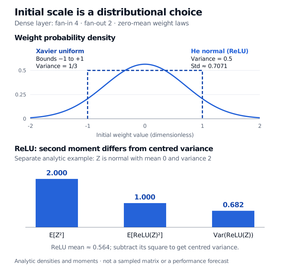
For our four-input, two-output layer, a=1: draw each weight from U(−1,1), whose variance is 1/3. The variance is a property of the sampling distribution. Eight drawn weights need not have exactly zero sample mean or sample variance 1/3.
Glorot and Bengio's derivation assumes independent initial weights and a locally linear regime for symmetric activations with derivative one at zero, as with tanh near zero. It is not an exact scale-preservation theorem for every sigmoid or softmax network. Even in the linear approximation, unequal fan counts make it a compromise: this example's forward variance multiplier is 4/3, while its backward multiplier is 2/3 under the corresponding independence assumptions.
ReLU changes the moment being tracked
He, or Kaiming, initialisation accounts for the rectified linear unit, ReLU(z)=max(0,z). Its fan-in normal form draws zero-mean weights with
Var(Wij)=fan-in2,Std(Wij)=fan-in2.
For fan-in 4, the variance is 0.5 and the standard deviation is approximately 0.7071. A normal distribution's second parameter in N(0,0.5) is variance, not standard deviation. Unlike the uniform example, these weights have no finite hard bounds.
With zero biases, symmetric zero-mean initial weights, and the independence assumptions used in He et al., §2.2, symmetric preactivations put half their second moment on either side of zero. ReLU retains only the positive side:
E[ReLU(Z)2]=21E[Z2].
That factor explains the doubled weight variance. It does not imply ReLU halves centred variance: its output generally has positive mean. As a separate exact example, if Z∼N(0,2), then
He scaling balances this second-moment propagation under the stated model, rather than forcing every activation's centred variance to equal its input's. A fan-out variant instead targets backward propagation. Leaky ReLU and PReLU require a gain reflecting their negative slope; the plain ReLU factor is not universal.
Analytic weight densities for fan-in 4 and fan-out 2: Xavier uniform has bounds minus 1 to plus 1 and variance one third; He normal has variance 0.5 and standard deviation about 0.7071. A separate normal Z with variance 2 has second moment 2; ReLU(Z) has second moment 1, mean about 0.564 and centred variance about 0.682.
Original analytic illustration, with dimensionless values. The curves describe weight distributions, not eight realised weights. The lower panel isolates the effect of ReLU in a separate Gaussian example.
Symmetry, orthogonality and identity
Randomness also helps otherwise interchangeable hidden units start differently. If hidden units have identical relevant incoming and outgoing parameters, identical activation functions and symmetric deterministic updates, they can continue learning the same function. Initialising an entire ordinary multilayer network to zero can create this failure. This is not a ban on zero-valued parameters: zero biases alongside distinct random weights are common. Deep Learning, §8.4, separates symmetry breaking from bias choices and discusses the competing risks of overly large and overly small weights. Structured schemes can deliberately start residual branches at zero, as the Fixup paper discusses. Their skip paths and other initial parameters make this a different construction.
Orthogonal initialisation introduces matrix structure instead of independent entries. A square orthogonal matrix Q satisfies Q⊤Q=I and preserves Euclidean norms before a nonlinear activation; a gain can rescale it. Rectangular constructions can only make rows or columns orthonormal, according to shape. Saxe et al. analyse why orthogonal starts can improve signal propagation, while making their linear-network and nonlinear-regime assumptions explicit. Norm preservation of one linear map does not guarantee well-behaved gradients for the whole trained network.
Identity initialisation is a specialised structured choice. Le, Jaitly and Hinton initialise the recurrent matrix of a ReLU recurrent network with the identity, or a scaled identity, to control how state persists. It is not a recipe to replace every dense weight matrix with an identity matrix.
Keep the starting point inside the research protocol
Inspect activation and gradient distributions on training data, and choose architecture, gain and initialisation through the permitted training and validation process. In financial time series, respect the information dates and keep the final test period out of those choices. A good initial scale cannot repair preprocessing leakage, unsuitable inputs or an incorrect objective.
Record the random seed, initializer, fan convention, architecture and software environment. A seed helps reproduce a draw; it does not establish robustness. If results vary materially across seeds, assess that variation using a predefined validation protocol rather than selecting the seed with the best final-test backtest. The reproducible MLP workflow connects seeds, tensor shapes, frozen preprocessing and chronological splits; its public preview leads to a membership lesson.