RMS normalisation rescales a vector of hidden activations by its root mean square, without subtracting its mean. Usually called RMSNorm, it gives a neural network a way to control representation scale while allowing its mean to remain nonzero. In an encoder for financial text or market sequences, that is an architectural choice about hidden features, rather than a procedure for estimating return volatility.
A scale computed from squares
For a group of hidden coordinates, write
Here is the uncentered second moment across the selected coordinates. It is not their variance: variance measures squared deviations from the mean. The positive constant protects the denominator at zero, while the learned gain adjusts each output coordinate.
This uses the epsilon-under-the-square-root convention documented by PyTorch RMSNorm and its current upstream implementation, checked on 1 November 2026. A denominator defines a different operation; record the exact convention when reproducing a model. Learned gains and additive biases also depend on the implementation: PyTorch's RMSNorm has optional gains and no additive bias parameter. Zhang and Sennrich's original paper, equation (4), defines RMS rescaling with gain, while equation (5) places a bias before the subsequent activation. Neither “always has a bias” nor “bias is forbidden” is a universal architectural rule.
The output can still be all positive
Take a synthetic dimensionless hidden vector . To isolate the arithmetic, use gain one and epsilon zero for this nonzero-RMS example only:
Its mean square is one, but its mean is approximately , not zero. Rescaling has preserved the positive direction of every coordinate. By contrast, layer normalisation subtracts the group's mean before dividing by a centred scale.
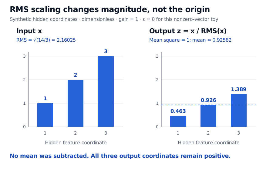
Original synthetic hidden-vector calculation. Values are dimensionless; the common vertical scale makes the rescaling visible. The dashed line marks the positive output mean, not a centring target.
With positive epsilon and gain one, the output mean square is , generally below one. Nonuniform learned gains can change it again. “RMS-normalised” therefore does not promise a final mean square of exactly one.
For nonzero vectors and epsilon zero, multiplying every input by the same positive constant leaves the normalised vector unchanged. Fixed positive epsilon breaks that exact scale invariance, though the difference becomes small when the squared signal scale dominates epsilon. Adding a common constant is not an invariance: it generally changes the vector's direction relative to the origin. A nonzero constant vector does not disappear as it would after mean subtraction.
Which coordinates share the denominator?
For a tensor with batch, time and feature axes, a common sequence-model choice computes one RMS across hidden features for each item at each time separately. No other batch member supplies that denominator. In contrast, training-time batch normalisation pools examples for each feature; layer normalisation uses a within-example group but also centres it. Extra spatial or temporal axes require an explicit decision, not an assumption based on the method's name. The Keras RMSNormalization documentation exposes this choice through its
axis argument.Feature-wise RMSNorm does not make an entire sequence model causal. A hidden vector may already contain future information, and pooling the denominator over future time positions can introduce look-ahead bias directly. Point-in-time inputs, causal sequence operations and chronological evaluation remain separate requirements. Rescaling hidden activations also does not replace training-only preprocessing of raw financial inputs with different units.
Finally, RMSProp is an optimiser, not an activation-normalisation layer: it accumulates squared gradients across training steps to scale parameter updates. See SGD, Momentum, RMSProp, and Adam as Optimization Choices (public preview; full lesson requires membership) for that distinction. Removing mean subtraction makes RMSNorm's statistic simpler than layer normalisation's; any runtime or forecasting benefit still needs measurement in the actual architecture and task.
Sources
- Zhang and Sennrich (2019), Root Mean Square Layer Normalization, §§3–4.1: RMSNorm's definition, gain, bias context and scale-versus-shift properties.
- PyTorch 2.9, RMSNorm, and current upstream RMSNorm source, checked 1 November 2026: denominator, reduction axes and gain configuration.
- Keras 3, RMSNormalization layer, LayerNormalization layer and BatchNormalization layer: selected axes and the distinct statistics used by these layers.
- Keras 3, RMSprop: moving squared-gradient statistics in an optimiser.