Improper integral: Definition & Examples

An improper integral is an integral defined by a limit because its interval extends to infinity or its integrand becomes unbounded near an endpoint or an interior point. First integrate over finite intervals that avoid the problem; then take the required limits. The integral converges only when those limits exist as finite real numbers. Otherwise it diverges.

In finance, this is the distinction between writing down an infinite-horizon valuation formula and proving that it has a finite value. It also matters when integrating a probability density over an unbounded range. MIT's introduction to improper integrals distinguishes an infinite interval from a singular integrand.

Begin with a finite horizon

Suppose a hypothetical contract delivers cash continuously at USD 100 per year, starting now and continuing forever. Assume a constant continuously compounded discount rate of

r=0.05

per year. Time

t

is measured in years, so

rt

is dimensionless. There is no default, changing cash rate or transaction cost in this model.

Through a finite horizon

T

, its present value is an ordinary definite integral:

V(T)=\int_0^T 100e^{-0.05t}\,dt =2000\left(1-e^{-0.05T}\right)\quad\text{USD}.

The integrand has units of USD per year; multiplying by $dt$ gives USD. Now let the horizon grow:

V=\int_0^\infty 100e^{-0.05t}\,dt :=\lim_{T\to\infty}V(T) =2000\quad\text{USD}.

Infinity is not a date at which to evaluate an antiderivative. The last step works because

e^{-0.05T}

tends to zero. More generally, a positive constant cash rate

c

has value

c/r

when

r>0

. At

r=0

, the finite-horizon value is

cT

and grows without bound. At

r<0

, the discount factor grows with time and the positive-stream integral also diverges. Substituting a negative rate into

c/r

would therefore give a meaningless negative valuation for this model.

Payment timing is part of the specification. This continuous stream is different from USD 100 delivered at each year-end: those payments require a geometric series with the appropriate discount convention. Neither construction guarantees that a real borrower can or will pay forever.

Convergence is not a cutoff rule

A computer cannot integrate to infinity. Even when convergence is established, a finite cutoff needs an error estimate. Here the omitted present value has an exact expression:

R(T)=\int_T^\infty100e^{-0.05t}\,dt =2000e^{-0.05T}\quad\text{USD}.

Cutoff $T$ (years)	Value included (USD)	Value omitted (USD)
20	1,264.24	735.76
40	1,729.33	270.67
60	1,900.43	99.57
100	1,986.52	13.48

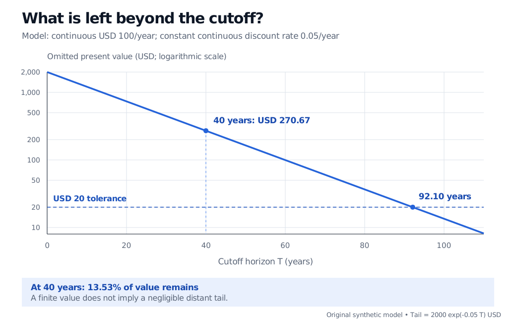
Forty years sounds distant, yet the remaining tail is 13.53% of the entire value. To omit at most USD 20, or 1% of USD 2,000, choose a horizon satisfying

2000e^{-0.05T}\le20 \quad\Longleftrightarrow\quad T\ge\frac{\ln100}{0.05}\approx92.10\text{ years}.

The cutoff must meet the unrounded bound; 92.10 years is its rounded display. This is a model calculation, not a recommendation to forecast cash flows with that precision.

Tail present value on a logarithmic USD axis for the hypothetical continuous USD 100 per year stream discounted at 0.05 per year. At 40 years USD 270.67 remains; the USD 20 threshold is reached at approximately 92.10 years.

Original synthetic model. The vertical axis is logarithmic, making exponential tail decay a straight line; its units are omitted present-value USD.

The general definition behind this example is

\int_a^\infty f(x)\,dx :=\lim_{B\to\infty}\int_a^B f(x)\,dx,

provided the finite-cutoff integrals exist and their limit is finite. A small value of $f(B)$ alone does not establish convergence or control the remaining area: $1/x$ tends to zero, but $\int_1^B dx/x=\ln B$ grows without bound.

A finite interval can still be improper

An endpoint blow-up requires a different cutoff. For $x^{-1/2}$ on $(0,1]$ ,

\int_0^1\frac{dx}{\sqrt{x}} :=\lim_{\varepsilon\downarrow0}\int_\varepsilon^1x^{-1/2}\,dx =\lim_{\varepsilon\downarrow0}2\left(1-\sqrt{\varepsilon}\right)=2.

The height becomes unbounded, but the area is finite. In contrast,

\int_0^1\frac{dx}{x} =\lim_{\varepsilon\downarrow0}(-\ln\varepsilon) =+\infty,

so that integral diverges. For powers, the useful distinction is: $\int_0^1x^{-p}\,dx$ converges for $p<1$ , whereas $\int_1^\infty x^{-p}\,dx$ converges for $p>1$ . At $p=1$ , both diverge. A mild singularity and a sufficiently fast-decaying distant tail are different requirements.

Check each problematic side separately

If an interval crosses a singularity, split there and require each one-sided integral to converge. Likewise, an integral over the entire real line requires convergence of both tails separately. OpenStax's definitions make this requirement explicit.

For $1/x$ on $[-1,1]$ , the left integral diverges to $-\infty$ and the right to $+\infty$ . Adding them is not a valid cancellation. The distinct, symmetric-cutoff calculation

\lim_{\varepsilon\downarrow0} \left(\int_{-1}^{-\varepsilon}\frac{dx}{x} +\int_\varepsilon^1\frac{dx}{x}\right)=0

is its Cauchy principal value; the ordinary improper integral still diverges. Absolute convergence, meaning finiteness of the corresponding integral of

\lvert f\rvert

, is stronger than ordinary convergence and rules out dependence on cancellation. A principal value requires its own definition and justification; a numerical routine returning zero is not enough.

For more methods and examples, the Improper Integrals lesson develops endpoint limits, power tests and comparison tests. Its public page is a preview; the full lesson requires membership.

Sources

James Stewart, Single Variable Calculus: Early Transcendentals, 6th edition, Brooks/Cole, 2008, §7.8, “Improper Integrals,” pp. 508–515.
MIT, 18.01, §27.1: When is an Improper Integral Finite?.
OpenStax, Calculus Volume 2, §3.7: Improper Integrals.

Begin with a finite horizon

Convergence is not a cutoff rule

A finite interval can still be improper

Check each problematic side separately

Sources

Related terms

Antiderivative

Definite integral

Geometric series

Present value

Probability density function