A geometric series adds terms obtained by repeatedly multiplying by the same number, called the common ratio. Its finite form is
Here is the first term and is the positive integer number of terms. For , read the terms directly as , with sum . A geometric sequence lists those terms; the series adds them. Unlike an arithmetic series, which uses a fixed difference, the geometric pattern uses a fixed multiplier.
In finance, this pattern appears when equal payments are discounted at a constant rate: each successive payment has the same fraction of the previous payment's present value. Recognising that ratio turns a long cash-flow sum into one expression.
A finite sum needs no convergence test
Multiply the sum by and subtract. All interior terms cancel:
This identity holds for any finite real , including negative ratios and ratios larger than one. When , every term is , so . A finite sum does not become invalid just because the corresponding infinite series would diverge.
The indexing matters: terms end at exponent . If the written sum ends at , it contains terms. MIT's introduction to series develops the distinction between individual terms and their running totals.
Five payments, all valued today
Suppose a hypothetical contract pays USD 100 at each year-end for five years, starting one year from today. Use a constant 5% annual effective discount rate, with the payments treated as certain and no tax or fees. This is a level annuity, not a principal repayment plus coupons.
The discount multiplier per year is
The payments themselves are equal. Their values today are geometric:
Thus the first term is , not 100, and the common ratio is , not 5%. Substitution gives
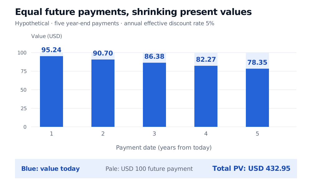
Original hypothetical cash-flow calculation. Pale bars show the USD 100 amounts paid on their respective future dates; blue bars show all five amounts valued today. Labels are rounded individually; the total uses unrounded values.
The answer is below the USD 500 nominal total because every payment is deferred and the stipulated rate is positive. The closed form already discounts every payment. Do not discount USD 432.95 again by five years: that would move an amount already valued today to the wrong date.
If the same five payments arrive at the beginning of each year, at dates 0 through 4, each is discounted for one fewer year. Their value is USD, or USD 454.60. OpenStax's annuity discussion explains this timing adjustment between an ordinary annuity and an annuity due.
At a zero rate, use the original sum: five payments are worth USD 500. The formula dividing by the rate has a removable zero-over-zero form there. For a finite stream, a negative rate above −100% is also mathematically admissible under annual effective compounding; do not apply the infinite-stream restriction to it.
Taking the number of payments to infinity
An infinite series means the limit of its partial sums, not a finite sum with an infinity symbol substituted for . For ,
The reason is that tends to zero exactly in this range. Negative ratios between −1 and 0 alternate in sign and still converge. At , nonzero partial sums oscillate; at , they grow in magnitude. For , the terms fail to approach zero. The exception is : the all-zero series converges to zero for every finite real ratio, including , where the fraction above is undefined. Stewart's §11.2 derives the result by partial sums with a nonzero first term.
If the USD 100 year-end payments continue forever under the same 5% assumption, the model becomes a perpetuity:
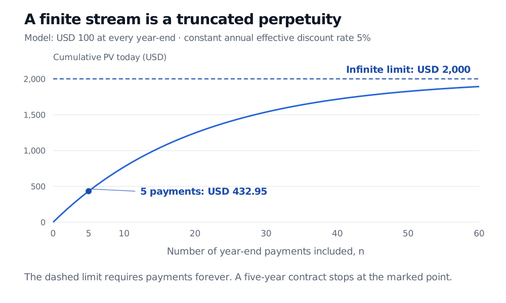
Original model partial sums, joined to show their shape. Only integer payment counts apply. The USD 2,000 line requires an unending stream; it is not the value of the five-year contract.
For this positive stream, a finite perpetuity value requires a positive annual effective rate: only then is . At zero rate the cumulative value grows by USD 100 per payment; at a negative rate above −100%, the discounted amounts grow rather than shrink. OpenStax's perpetuity chapter treats the perpetual-payment assumption explicitly.
When the shortcut stops fitting
Use the geometric formula only after checking the pattern in the amounts being summed. Irregular payment dates, changing payments or a nonconstant discount curve generally break the constant ratio. Then value each dated cash flow with its applicable discount factor and add the results. The finite-sum identity remains exact; the question is whether the financial inputs actually have that form.
For a deeper mathematical treatment, Series and the Geometric Series: Partial Sums and Convergence develops running totals, telescoping and the divergence test. The public page is a preview; full reading requires membership.
Sources
- James Stewart, Single Variable Calculus: Early Transcendentals, 6th edition, Brooks/Cole, 2008, §11.2, “Series,” especially Example 1 and the geometric-series formula, pp. 688–690.
- MIT OpenCourseWare, 18.01SC Single Variable Calculus, “Introduction to Series”.
- OpenStax, Principles of Finance, §8.2, “Annuities”.
- OpenStax, Principles of Finance, §8.1, “Perpetuities”.