Why stocks with high past residual volatility can earn low subsequent returns, and how factor models, lottery payoffs and implementation change the evidence.
Idiosyncratic volatility anomaly
The idiosyncratic volatility anomaly is the empirical pattern that stocks with high previously measured residual return volatility have subsequently earned unusually low average returns in some equity samples and portfolio constructions. It matters when a quant uses stock-specific volatility as a trading signal: a larger unexplained risk estimate does not automatically imply a larger expected reward.
The anomaly is a statement about returns after a sort. Idiosyncratic risk is the underlying risk concept; residual volatility is a way to measure it relative to specified factors. A low-total-volatility stock selection and a low-residual-volatility selection can choose different companies.
First remove the modelled exposures
A typical measurement starts with a time-series regression of daily excess stock returns on factor returns:
ri,d=αi+bi⊤fd+ϵi,d.
Here ri,d is the stock return less the risk-free return, fd contains the chosen factors, and ϵi,d is the unexplained component. Fit the coefficients over a stated historical window, then measure the dispersion of the fitted residuals. For example, with n usable observations and K factors, an ordinary least squares residual standard-error convention is
σϵ,i=n−K−1∑d=1nϵi,d2.
This formula assumes an intercept, full column rank and n>K+1. It specifies a convention, rather than a universal definition of every published IVOL series: residual sample SD and root mean squared residual can use different denominators. Record that choice when reproducing a study.
The factor set determines what remains unexplained. Adding industry or style exposures can remove variation previously counted as residual risk. Window length, daily versus monthly observations, missing prices, thin trading and the small number of observations in a short window also affect the estimate and the ranking.
A trailing residual SD is a historical statistic. A volatility forecast instead targets uncertainty conditional on information available now. Using a conditional forecast, contemporaneously realised volatility, or next month's residuals changes the question; next month's residuals cannot be used to form an investable sort today.
A risk split cannot establish a return anomaly
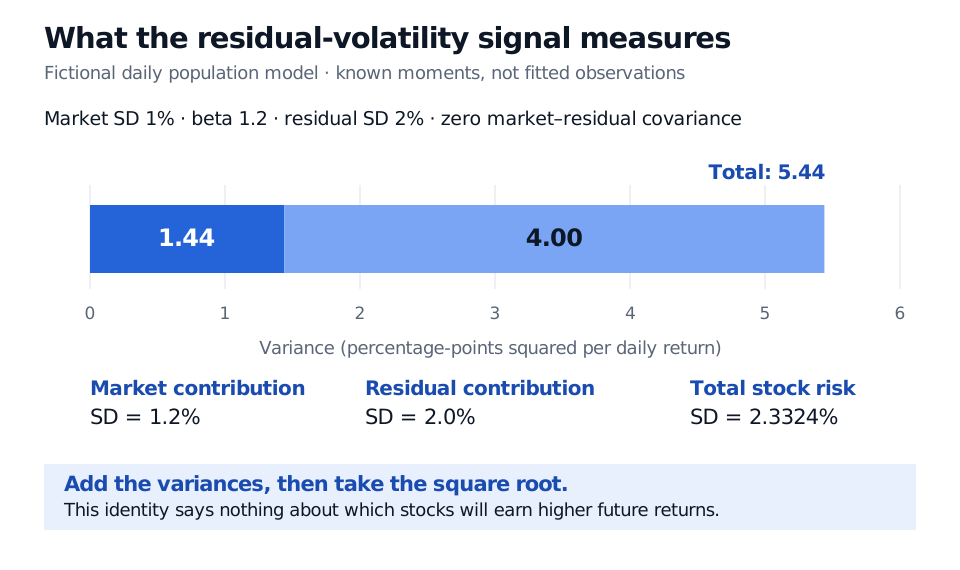
Consider a fictional daily population model with market SD 1%, stock market loading 1.2, residual SD 2%, and zero covariance between market and residual returns. These are known moments, not estimates from a handful of observations. Its variance is
so total daily SD is 0.000544≈2.3324%. The residual SD remains 2%. The market contribution has SD 1.2%; adding 1.2% and 2% would incorrectly add standard deviations instead of variances.
Fictional daily population model: systematic variance 1.44 plus residual variance 4.00 equals total variance 5.44 in percentage-points squared. The component SDs are 1.2% and 2.0%, and total SD is 2.3324%.
Original fictional known-moment example. Variances add because the market and residual are uncorrelated; the calculation supplies no future-return ranking.
Nothing in this identity determines the stock's expected return. Even the idealised argument that diversifiable risk earns no separate risk premium does not predict a negative premium. The anomaly requires separate return evidence.
What the original finding actually compared
Ang, Hodrick, Xing and Zhang (2006), §II and Table VI panel B, measured residual volatility relative to the Fama–French three-factor model. Their baseline US-stock experiment estimated it from daily returns in the previous month, formed value-weighted quintiles, and held them for the next month, rebalancing monthly.
For July 1963–December 2000, the lowest-IVOL quintile's average monthly total return was 1.04%, versus −0.02% for the highest. High minus low was therefore −1.06 percentage points per month. The corresponding three-factor alpha difference was −1.31 percentage points per month. Raw returns and model-adjusted alphas answer different questions. These historical estimates are neither a promised spread nor proof that increasing a firm's volatility causes its return to fall.
Why the specification travels with the result
Bali and Cakici (2008), abstract, report that data frequency, portfolio weighting, sorting breakpoints and size, price and liquidity screens materially affect the relationship. Their alternative constructions do not produce a robustly significant relation. Treat that as evidence about sensitivity, rather than a universal verdict that every IVOL study must agree.
A possible economic channel is demand for lottery-like stocks: investors may bid up shares with attractive extreme positive payoffs, reducing subsequent expected returns. Residual volatility measures dispersion, whereas skewness concerns asymmetry; one is not a substitute for the other. Bali, Cakici and Whitelaw (2011), §3 and Tables 9–10, study MAX, the largest daily return in the previous month. Their controls substantially change the IVOL relation, but the simple value-weighted double sort retains a negative IVOL spread. This is a competing interpretation with specification-dependent evidence, not a settled causal explanation.
For a trading implementation, inspect how much of a result comes from microcaps or low-priced shares and whether the intended positions can trade. Wide spreads and market impact can consume a paper spread. The high-IVOL short leg also needs borrow availability, borrow fees and capacity checks; violent positive jumps can hurt it while leaving a long-run average relationship intact. Include delisting returns and a universe known at each formation date. Report gross and net results separately, with a holding period and weighting rule that match the tested signal.
For the underlying risk algebra, Sharpe's Single-Index Model derives the variance split and explains residual-risk diversification. Its public preview is available; the full lesson requires membership. The derivation helps identify the measured component before asking whether that component predicts returns.