Hyperbolic sine, cosine and tangent combine opposite exponentials. See their identities, calculus and why equal opposite log shocks do not average to an unchanged price.
Hyperbolic function
A hyperbolic function is a function built from combinations of the exponentialsex and e−x. The main three are hyperbolic sine, hyperbolic cosine and hyperbolic tangent. They separate a pair of opposite exponential changes into a symmetric part and a signed part—a useful distinction when converting log-return scenarios into prices.
For a real, dimensionless input x,
sinhx=2ex−e−x,coshx=2ex+e−x,tanhx=coshxsinhx.
These are the standard NIST definitions. Read the names as “hyperbolic sine,” “hyperbolic cosine” and “hyperbolic tangent.” The extra h matters: these are different functions from sin, cos and tan.
What the three shapes tell you
Function
Symmetry
Range for real input
Value at zero
coshx
Even: cosh(−x)=coshx
[1,∞)
1
sinhx
Odd: sinh(−x)=−sinhx
All real numbers
0
tanhx
Odd: tanh(−x)=−tanhx
(−1,1)
0
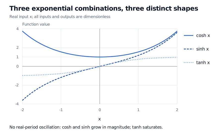
Hyperbolic cosine averages the two exponentials, so reversing the sign of x changes nothing. Hyperbolic sine takes half their difference, so reversing x reverses its sign. Their ratio, hyperbolic tangent, increases smoothly toward 1 or −1 but never reaches either at a finite real input.
On the real interval minus 2 to 2, cosh is an even U-shaped curve with minimum 1; sinh is an odd increasing unbounded function; tanh is odd and increases between horizontal limits minus 1 and 1.
Original mathematical curves. Inputs and function values are dimensionless; the plotted interval is only part of each function's domain.
The family also includes reciprocal functions: sechx=1/coshx, cschx=1/sinhx and cothx=coshx/sinhx. The last two are undefined at x=0.
You can derive it directly: put a=ex and b=e−x. Then
(2a+b)2−(2a−b)2=ab=1.
For real inputs, none of sinh, cosh or tanh repeats with a nonzero real period. In particular, tanh is a saturating curve, not an oscillating tangent wave. Statements about imaginary periods belong to their complex extensions.
Two other useful identities reconstruct the original exponentials:
ex=coshx+sinhx,e−x=coshx−sinhx.
Equal log shocks do not average to an unchanged price
Start with a synthetic price of USD 100 and two alternative scenarios at the same future horizon. Assume positive prices and no intervening cash distributions. A price log-return is r=ln(S1/S0), so S1=S0er; the logarithm reverses the exponential transformation.
Give the two scenarios equal weight and choose r=+0.2 and r=−0.2. These are log-return units, not simple returns of plus and minus 20%.
Scenario
Terminal price, USD
Simple price return
r=+0.2
100e0.2=122.140276…
+22.140276…%
r=−0.2
100e−0.2=81.873075…
−18.126925…%
The average log-return is zero. The arithmetic average price is
Here 100sinh(0.2) is half the difference between the scenario prices, while tanh(0.2) is their difference divided by their sum. These interpretations follow from the definitions; they do not assign probabilities to the scenarios.
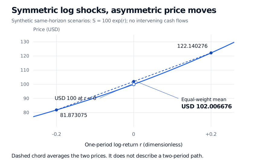
A convex synthetic price curve S equals 100 exp(r). At log-return minus 0.2 the price is USD 81.873075; at plus 0.2 it is USD 122.140276. The dashed chord midpoint is their equal-weight mean, USD 102.006676, above USD 100 at zero log-return.
Original synthetic same-horizon scenarios, with no intervening cash flows. The dashed chord averages two alternative terminal prices.
The gap arises because the exponential is a convex function: equal opposite changes in its input produce unequal changes in its output. The geometric mean of the two prices is exactly (100e0.2)(100e−0.2)=100. The arithmetic mean exceeds it.
Alternative scenarios are different from consecutive returns. A price that experiences +0.2 and then −0.2 as consecutive log-returns returns to 100e0.2e−0.2=100, under the same no-distribution assumption. USD 102.006676 is the average across two alternative endpoints, not the result of that round trip. Equal scenario weights also do not establish a real-world expected gain or alpha. Actual probabilities, financing and a trading rule would require separate assumptions.
Unlike the derivative of ordinary cosine, the derivative of hyperbolic cosine has no minus sign. These formulas are listed in NIST's derivative reference. Since cosh′′x=coshx>0, hyperbolic cosine is strictly convex everywhere. Meanwhile the slope of tanh tends to zero near its limiting levels: bounding an output with tanh also compresses changes in large inputs.
Odd powers cancel from the exponential average. Consequently the leading increase in the equal-weight mean price is quadratic in shock size: 100coshx≈100(1+x2/2). At x=0.2 this approximation is USD 102, close to the exact USD 102.006676. It explains the curvature effect without treating the approximation as an exact pricing model.
For the exponential and log-return prerequisites, Exponentials and Logarithms develops the price transformation and aggregation through time. The public page is a preview; the full lesson requires membership.
Sources
Stewart, J. (2008). Single Variable Calculus: Early Transcendentals, 6th edition, §3.11, “Hyperbolic Functions,” pp. 254–258. Brooks/Cole.