Measure departure from unimodality using empirical CDF distance, interpret the uniform reference, and avoid confusing a dip statistic with a mode count or normality test.
Hartigan dip test
The Hartigan dip test is a nonparametric hypothesis test of whether a one-dimensional population distribution is unimodal. In quantitative research, it can flag a return, spread or model-score distribution that deserves closer inspection before it is summarised by one central peak. It does not identify market regimes or tell you how many clusters to trade.
The statistic asks how closely the sample's cumulative distribution can be approximated by a unimodal cumulative distribution. It avoids choosing histogram bins or a density-estimation bandwidth. Its name refers to a distributional discrepancy, not the depth of a valley in a plotted histogram. Hartigan's original algorithm paper describes this construction.
The distance being measured
Let Fn be the empirical distribution's cumulative distribution function and let U be the class of unimodal CDFs. The dip functional is
D(Fn)=G∈Uinfxsup∣Fn(x)−G(x)∣.
The inner operation finds the largest vertical discrepancy for a candidate G; the outer operation chooses the best unimodal candidate. The result is measured on the probability scale, rather than in return units. For a continuous density, unimodality means the density rises toward a mode and falls afterwards, allowing flat portions. Correspondingly, its CDF is convex before the mode and concave after it. It need not be symmetric or bell shaped.
This is a shape restriction, not a test of the normal distribution. A skewed unimodal population can satisfy the null. Neither rejection nor non-rejection establishes Gaussianity.
Eight observations, one descriptive statistic
Consider these eight fictional measurements of a continuous variable, in illustrative units:
0,0.1,0.2,0.3,4,4.1,4.2,4.3.
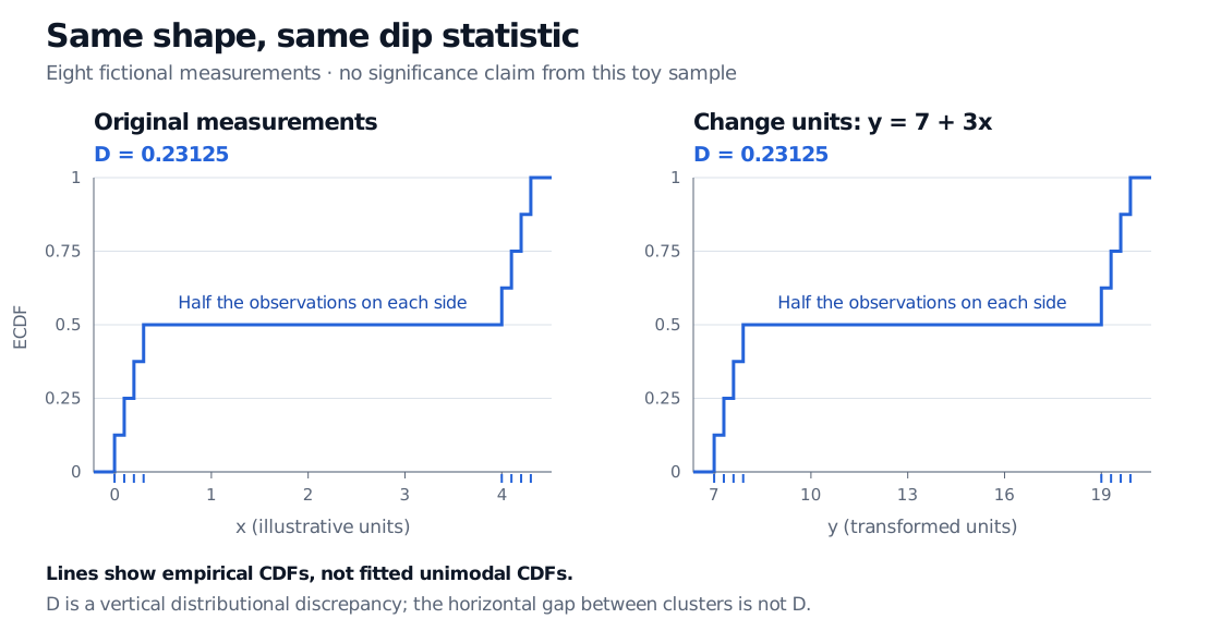
Four observations are at or below 0.3, so F8(0.3)=0.5. No observations fall between 0.3 and 4, leaving a long plateau between two steep sections of the empirical CDF.
The dipstat routine in Python diptest 0.12.0, with allow_zero=True, reports D=0.23125. Transforming every observation by y=7+3x leaves that statistic unchanged. More generally, positive affine transformations preserve the unimodality restriction and vertical CDF distances. A nonlinear transformation can change distributional shape; this invariance does not extend to arbitrary changes of scale.
Two empirical CDFs for eight fictional measurements, before and after y equals 7 plus 3x. Both report dip D equals 0.23125 in diptest 0.12.0 with allow_zero True; half the observations lie on either side of each long plateau.
The horizontal gap changes units, while the dip statistic stays the same. The plotted curves are empirical CDFs, not fitted unimodal CDFs; the plateau's width is not the dip statistic.
Report the implementation and minimum-statistic convention with reproducible results. The R package manual documents a different default, min.is.0=FALSE, which imposes a minimum of 1/(2n). These conventions can differ in exceptional samples. They give the same value for this example.
Turning a statistic into evidence
A larger dip means a larger discrepancy, but D is not a p-value. The usual test compares it with reference values from independent uniform samples of the same size. Uniform calibration reflects an asymptotically least favourable unimodal reference; it does not mean the null says the population must be uniform. Official implementations offer tabulated interpolation or uniform Monte Carlo calibration. A simulation report should state the replicate count and random seed, as well as the statistic convention.
No p-value is assigned to the eight-observation illustration here. Its purpose is to show the statistic and its invariance. It supplies neither a reliable mode count nor an explanation for the apparent separation. Non-rejection in a small sample may simply reflect weak power; rejection points to a failure of unimodality under the test's assumptions, rather than proving exactly two peaks.
For financial data, the sampling design matters. Standard calibration assumes independent, identically distributed observations; serially dependent returns or overlapping windows need a separately justified calibration. Tick sizes and rounded scores create ties, so a continuous reference may misrepresent their sampling behaviour. Keep the ties visible and justify the measurement model instead of silently adding random jitter. Searching many assets, windows or transformations also changes the meaning of the smallest reported p-value. These are parts of the research design, not defects a small dip statistic can resolve.
To work through the step function behind the statistic, see The Empirical CDF, Glivenko–Cantelli, and QQ-Plots. The public preview outlines the lesson; full teaching and worked exercises require membership.