A geometric Asian option uses a geometric average of scheduled prices. See its payoff, the role of correlated log-prices, and its use as a Monte Carlo benchmark.
Geometric Asian option
A geometric Asian option is an Asian option whose payoff uses the geometric mean of specified underlying-price observations. It averages log-prices and then exponentiates. That choice makes it especially useful as an analytical benchmark and as a control for Monte Carlo pricing of arithmetic Asian options. Replacing an arithmetic average with a geometric average changes the cash flows of the contract.
For n equally weighted positive fixings at times t1,…,tn, the mean is
G=(i=1∏nSti)1/n=exp(n1i=1∑nlogSti).
The observation schedule specifies which prices enter the product. Neither the initial price nor the expiry price enters automatically. The logarithmic definition requires strictly positive observations; it cannot be carried unchanged into a model that permits zero or negative prices.
A small change in the average can change exercise
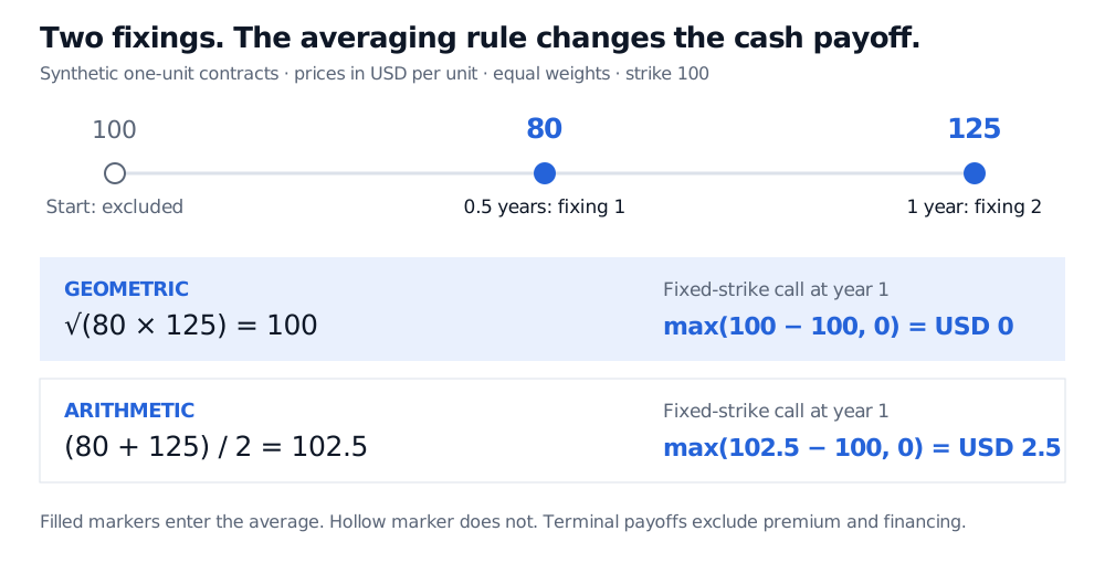
Take two equally weighted fixings, 80 at half a year and 125 at one year, quoted in USD per underlying unit. The starting price is 100 and is excluded. A synthetic European fixed-strike call covers one unit, has strike K=100, and pays cash at year 1.
G=80×125=100,A=280+125=102.5.
The geometric call pays (G−K)+=0. The corresponding arithmetic call pays (A−K)+=2.5, or USD 2.50 for the one-unit exposure. Here (x)+=max(x,0). These are terminal payoffs, excluding premium and financing; a zero payoff does not mean the option had zero value when written.
Two equal scheduled fixings, 80 and 125, give geometric mean 100 and arithmetic mean 102.5. A fixed-strike call with strike 100 pays USD 0 or USD 2.5 respectively at year 1; the starting price 100 is excluded.
Original synthetic example in USD per underlying unit. Filled markers are the two equal-weight fixings; the hollow starting observation is excluded. Both one-unit fixed-strike calls settle at year 1.
For identical positive observations, the arithmetic–geometric mean inequality gives G≤A. Applying the fixed-call payoff therefore gives
(G−K)+≤(A−K)+.
This is a pathwise bound, so it also orders their values when both are valued under the same risk-neutral model, discounting and otherwise matching terms. Equality of payoffs can occur even when the means differ: both calls may finish below strike.
The strike rule matters. A fixed-strike geometric put pays (K−G)+ and has the reverse inequality against its arithmetic counterpart. A floating-strike geometric call pays (ST−G)+; lowering the mean lowers its strike, so it pays at least as much as the matching arithmetic floating-strike call. The word “geometric” specifies the average, rather than specifying fixed versus floating strike.
Why correlated fixings still give a closed form
Under a constant-parameter geometric Brownian motion model, the vector of fixing log-prices is jointly normal. Its average is therefore normal, making Glognormal. Independence between fixing levels is unnecessary: prices on one path share earlier shocks.
To see exactly where the dependence enters, suppose all fixings are still in the future, 0<t1<⋯<tn≤T, and under the risk-neutral measure,
logSt=logS0+(r−q−2σ2)t+σWt.
Here r is the constant continuously compounded risk-free rate, q a constant continuous dividend yield, σ constant volatility and Wt Brownian motion. Prices use one fixed quote unit and times are in years. With tˉ=n−1∑iti, write logG∼N(m,v), where
The double sum comes from Cov(Wti,Wtj)=min(ti,tj). Dropping its off-diagonal terms would incorrectly treat the observations as independent and understate log-average variance. More generally, marginal lognormality of each price alone is insufficient; the joint distribution matters. Glasserman develops this reduction in §3.2.2, pp. 99–100.
For a European fixed-strike call paying at T, with K>0 and v>0, direct integration of this lognormal payoff gives
where Φ is the standard normal cumulative distribution function. If v=0, use the deterministic payoff e−rT(em−K)+ instead. This formula is exact within the stated model and fixing schedule, rather than a model-free market price. Known past fixings, nonconstant parameters or another price process require the corresponding conditional distribution or a different calculation. Back, Liu and Loewenstein give discrete- and continuous-sampling geometric-Asian valuations.
A benchmark that helps price a different contract
In Monte Carlo simulation, compute the discounted arithmetic and geometric call payoffs on the same simulated paths, using the same fixings. The geometric payoff's analytically known expectation can then anchor a control variate, reducing sampling noise when the payoffs are sufficiently correlated. The arithmetic payoff remains the pricing target. Simply reporting the geometric price instead leaves a contract-substitution error that more paths cannot remove.
Monte Carlo Option Pricing develops the control-variate estimator and its variance calculation. The link opens a public preview; the full lesson requires membership.
Two final distinctions prevent mismatches. A weighted geometric mean is Gw=exp(∑iwilogSti) for nonnegative weights summing to one; equal-weight formulas cannot silently be reused with unequal weights. A continuously sampled geometric mean over [0,T] is exp(T−1∫0TlogStdt); its moments differ from those of a finite fixing calendar. Specify the weights and schedule before choosing a valuation formula.
Sources
John C. Hull, Options, Futures, and Other Derivatives, 9th Global Edition, Pearson, 2018, §26.13, pp. 631–633, especially footnote 10 on p. 632: geometric versus arithmetic averaging under GBM.