Lower partial moments combine shortfall frequency and severity below a chosen return target. See general orders, all-observation weighting, units and target sensitivity.
General-order lower partial moments
General-order lower partial moments (LPMs) measure the expected powered shortfall of a return below a chosen target. They let a quant distinguish the chance of missing an objective from the size of the miss and the extra weight assigned to severe misses. Returns above the target contribute zero, even if they are unusually large.
The target and the order are separate choices: the target defines failure; the order determines how shortfall severity enters the calculation. A zero target asks about losing money. A positive target can classify a profitable outcome as a shortfall.
One family, several questions
Let R be a return over a specified horizon and τ a fixed target in the same return units and over the same horizon. For any real order p>0, define
LPMp(τ)=E[((τ−R)+)p],(x)+=max(x,0),
provided that this expectation is finite. Equivalently, integrate (τ−r)p over the part of the return distribution below τ. This is a moment of the nonnegative shortfall, rather than a central moment of the original return.
Order
What it measures
p=1
Expected shortfall amount below the target, including zero shortfalls.
p=2
Target semivariance: the expected squared shortfall. Its square root is target downside deviation.
Other positive p
A different severity weighting; fractional orders are permitted.
The zeroth-order member needs its own convention. Here it is strict shortfall probability:
LPM0(τ)=P(R<τ).
Do not insert p=0 mechanically into the positive-part formula: above-target outcomes then involve 00. If a source instead counts R≤τ, it includes outcomes exactly at the target. The distinction matters for discrete scenarios and rounded observations; it disappears for distributions with no probability mass at τ.
Maasar, Roman and Date, Section 2, give the target LPM family and its first- and second-order interpretations. Unser, Section 2.2, discusses target choice and the special cases. Mean-centred semivariance is the special choice τ=E[R]; an arbitrary target semivariance need not use the mean.
A 20% chance of a 10% loss
Consider a fictional one-month simple-return model with three possible outcomes. These are assumed probabilities, not a historical sample or forecast.
The model has a 20% shortfall probability, an expected shortfall amount of 2 percentage points, and downside deviation0.002≈0.04472136, or 4.47214 percentage points. The second moment itself has squared-return units: it is not a 0.2% loss probability or a 0.2% downside deviation.
The first moment's 2 percentage points is not the average loss when a loss occurs. Conditional on a shortfall, the miss is always 10 percentage points. For positive shortfall probability,
LPMp(τ)=P(R<τ)E[(τ−R)p∣R<τ].
This decomposition preserves both frequency and severity. In an equally weighted sample, estimate the LPM by dividing the sum of powered shortfalls by all n observations, including zeros. Dividing only by the number of shortfalls estimates the conditional expectation instead.
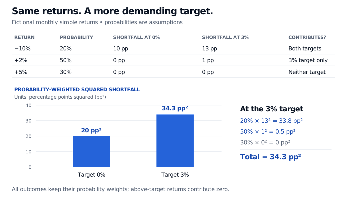
Now raise the monthly target to 3%. The −10% return misses it by 13 percentage points; the +2% return misses it by one. Thus
LPM2(0.03)=0.20(0.13)2+0.50(0.01)2=0.00343.
The shortfall probability rises to 70%. The return distribution did not deteriorate: the required outcome became more demanding.
Fictional monthly returns minus 10, plus 2 and plus 5 percent have probabilities 20, 50 and 30 percent. Raising the target from zero to 3 percent increases the second lower partial moment from 20 to 34.3 percentage points squared.
Original fictional monthly scenario. At the 3% target, weighted squared contributions are 33.8, 0.5 and zero percentage points squared. These sum to 34.3, equivalent to 0.00343 in decimal-return-squared units.
Higher order means greater relative emphasis on large misses
For two positive shortfalls sa>sb, their penalty ratio is (sa/sb)p. A 4 percentage point miss receives four times the penalty of a 1 percentage point miss at p=1, but sixteen times at p=2. For 0<p<1, the penalty grows sublinearly; for p>1, it grows superlinearly.
This does not mean the raw LPM must rise as the order rises. In the example, 0.002<0.02: powers of decimal shortfalls below one get smaller, and the units change with p. Converting returns from decimals to percentage-point numbers multiplies LPMp by 100p. Compare portfolios using the same order, target, horizon and unit convention. Taking the pth root restores return units, but it does not remove the economic choice of order.
Connect it to the risk question
The Sortino ratio uses LPM2(τ) in its denominator under the all-observation convention, with mean return above the target in its numerator. LPMs themselves are downside summaries, not performance ratios. The first-order target shortfall is also distinct from Expected Shortfall, which averages losses over a specified worst probability fraction.
The same mathematics can be written on the loss side. If L=−R and q=−τ, then (τ−R)+=(L−q)+: a return-side lower partial moment becomes a loss-side upper partial moment. The membership lesson Expected Shortfall and Other Tail Risk Measures develops upper partial moments and their stop-loss interpretation in Section 5.2; its public page provides a preview.
Keep the measurement horizon explicit. There is no general square-root annualisation rule for downside deviation: the shortfall of a compounded annual return is not the sum of monthly shortfalls. Estimate the chosen horizon's return distribution against that horizon's target. A larger order also places greater weight on rare severe misses, making a finite sample especially vulnerable to missing those outcomes. A finite empirical LPM does not establish that the population moment is finite.
Finally, LPMs ignore the ordering of an identical set of returns and all gains above the target. They cannot tell the full story about upside potential, funding needs or maximum drawdown. Their usefulness comes from stating precisely which downside question they answer.
Practice: a return exactly at target
Four one-month simple returns are equally likely: −3%, 0%, +1% and +6%. At a fixed monthly target of +1%, what are the strict shortfall probability and second LPM in decimal-return units? What is the downside deviation?
Answer. The first two outcomes miss the target, giving probability 2/4=50%. The +1% outcome exactly meets it and contributes zero. The shortfalls are 0.04,0.01,0,0, so LPM2(0.01)=(0.042+0.012)/4=0.000425. Downside deviation is 0.000425≈0.02061553, or 2.06155 percentage points. Dividing by two would remove the zero-shortfall observations and produce a conditional second moment instead.