Fixed-point iteration: Definition & Examples

Fixed-point iteration is the algorithm that repeatedly applies a chosen function to its current estimate:

x_{k+1}=g(x_k),\qquad k=0,1,2,\ldots.

Its target is a fixed point, a value

x^*

satisfying

g(x^*)=x^*

. In financial calibration, an equation can often be rearranged into this form. The rearrangement chooses the algorithm: two maps can encode the same desired price or parameter and produce entirely different numerical behaviour.

If the iterates converge to

x^*

and

g

is continuous there, taking limits in the update gives

g(x^*)=x^*

. That observation identifies a possible limit; it does not establish that the iteration will converge. Driscoll and Braun’s treatment makes the choice of map central to the method.

One equation, two update rules

Take the dimensionless equation $x^2=2$ and restrict attention to $x>0$ . Both

g(x)=\frac{1}{2}\left(x+\frac{2}{x}\right) \quad\text{and}\quad h(x)=\frac{2}{x}

have the unique positive fixed point $\sqrt{2}$ . Their iterations behave differently.

For $g$ , starting at $x_0=3/2$ gives:

$k$	Exact $x_k$	Decimal, rounded
0	$3/2$	1.500000000
1	$17/12$	1.416666667
2	$577/408$	1.414215686
3	$665857/470832$	1.414213562

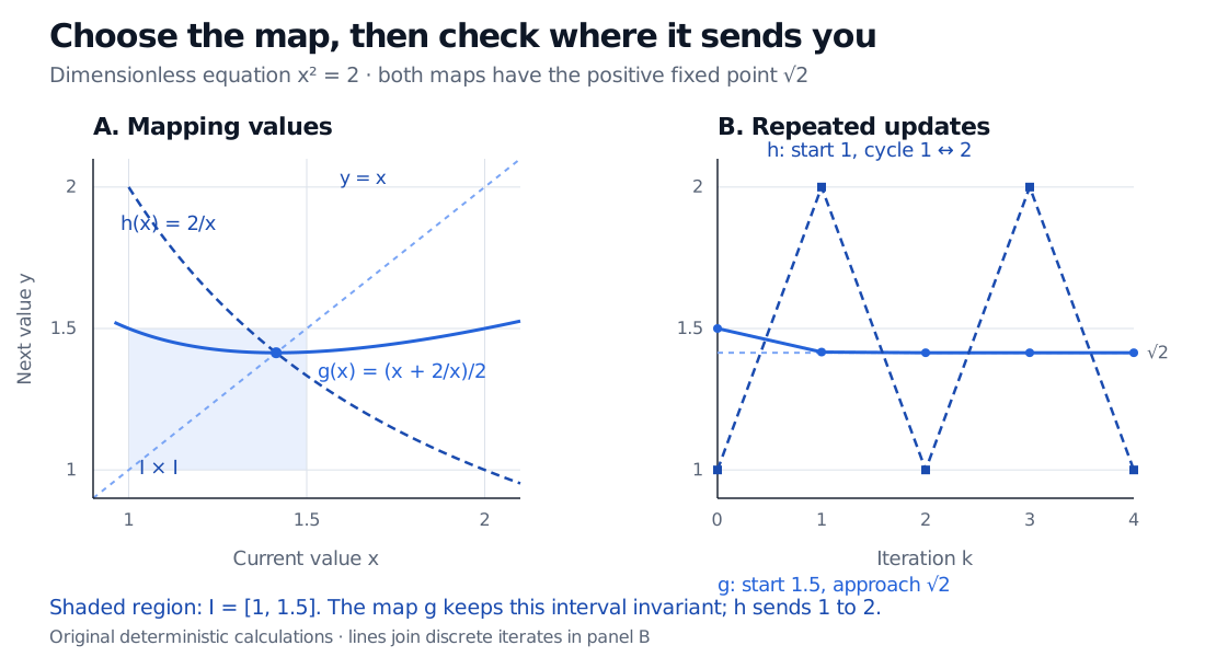
For $h$ , starting at $x_0=1$ gives $1,2,1,2,\ldots$ . In fact, $h(h(x))=x$ for every positive $x$ . Unless the starting value is already $\sqrt{2}$ , the iteration returns to its starting value every two steps.

The first map is exactly the Newton–Raphson update for

f(x)=x^2-2

. Fixed-point iteration is the broader construction; it need not use derivatives or Newton’s tangent rule. Stewart’s §4.8 develops that particular root-finding update.

The map g keeps the interval from 1 to 1.5 invariant and iterates from 1.5 approach square root of 2. The map h sends 1 to 2 and cycles between those two values.

Original deterministic comparison for $x^2=2$ , with dimensionless coordinates. The shaded region is $I\times I$ for $I=[1,1.5]$ ; the graph of $g$ over $I$ stays inside it. Panel B joins discrete iterates: $g$ starts at 1.5, while $h$ starts at 1.

A guarantee needs a domain as well as a slope

A useful scalar version of the contraction mapping theorem starts with a closed interval

I=[a,b]

and two checks:

Invariance: $g(I)\subseteq I$ , so updates cannot escape the interval.
Uniform contraction: some constant $0\le q<1$ satisfies $\lvert g(x)-g(y)\rvert\le q\lvert x-y\rvert$ for every $x,y\in I$ .

Then there is exactly one fixed point in

I

, and iteration converges to it from every

x_0\in I

. For a continuously differentiable scalar map, a sufficient way to check the second condition is

\sup_{x\in I}\lvert g'(x)\rvert\le q<1

. The mean value theorem supplies the distance bound. LeMesurier’s notes distinguish these interval and derivative requirements.

For our $g$ , choose $I=[1,3/2]$ . Its minimum on this interval is $\sqrt{2}$ and its maximum is $3/2$ , so it maps $I$ back into $I$ . Also,

g'(x)=\frac12-\frac{1}{x^2},\qquad -\frac12\le g'(x)\le\frac1{18}\quad(x\in I).

Thus

q=1/2

works. This proves convergence from every starting value in that interval, rather than merely observing several successful updates. Uniqueness is a claim within

I

and the positive branch; the original equation also has the negative root

-\sqrt{2}

A derivative test at the fixed point answers a narrower question. If $g$ is continuously differentiable near $x^*$ and $\lvert g'(x^*)\rvert<1$ , sufficiently close starts converge. It does not certify a distant start or a large proposed interval. Here $g'(\sqrt{2})=0$ ; the exact error identity, with $e_k=x_k-\sqrt{2}$ , is

e_{k+1}=\frac{e_k^2}{2x_k}.

That explains why this particular iteration eventually improves much faster than the conservative factor

1/2

permits. See convergence of a numerical method for the distinction between a rate and a guarantee about allowed starts. Bindel’s Cornell notes develop both contraction bounds and local behaviour.

These are sufficient conditions, not necessary conditions for every convergent iteration. For example, $u_{k+1}=u_k/(1+u_k)$ from $u_0=1$ has $u_k=1/(k+1)\to0$ , although the map’s derivative at its fixed point is $1$ . No uniform contraction factor below one works on $[0,1]$ .

Turning a small step into a useful bound

When the invariant-interval contraction conditions hold, the unseen future steps form a bounded geometric tail. In exact arithmetic, for $k\ge1$ ,

\lvert x_k-x^*\rvert \le \frac{q}{1-q}\lvert x_k-x_{k-1}\rvert.

For $q=1/2$ , the multiplier is one. The table’s $x_2$ is therefore within $\lvert x_2-x_1\rvert=1/408$ of the root. This bound is valid but conservative: its actual error is about $2.124\times10^{-6}$ .

The multiplier matters. If the only established factor is

q=0.999

, it becomes

999

. A small successive change alone is therefore no accuracy certificate. Without a proven bound, it may reflect slow progress or floating-point stagnation. A rounded zero step does not inherit the exact-arithmetic guarantee automatically.

For a calibration calculation, monitor the original equation’s residual, domain validity and an iteration limit alongside the step size. Choose a map whose fixed points really correspond to the intended solution on the admissible domain. Multiplying or dividing an equation can change that domain or introduce unwanted solutions.

SelfMadeQuant’s Root-Finding and Numerical Integration shows how a bond-yield equation leads to Newton’s update and why a bracket can provide a safeguard. The full lesson requires membership; its outline and introduction are publicly previewable.

Sources

Driscoll, T. A., and Braun, R. J., Fundamentals of Numerical Computation, §4.2, “Fixed-point iteration.”
LeMesurier, B., Numerical Methods and Analysis with Python, §1.2, “Solving Equations by Fixed Point Iteration (of Contraction Mappings).”
Bindel, D., Cornell CS 4220, “Fixed point iteration and Newton,” 27 March 2026.
Stewart, J. Single Variable Calculus: Early Transcendentals, 6th ed., Thomson Brooks/Cole, 2008, §4.8, pp. 334–337.

One equation, two update rules

A guarantee needs a domain as well as a slope

Turning a small step into a useful bound

Sources

Related terms

Convergence of a numerical method

Fixed point

Floating-point arithmetic

Newton-Raphson method

Residual