Expected maximum drawdown averages each path’s worst peak-to-trough loss. See why it differs from drawdown of an average path, and why horizon and modelling matter.
Expected maximum drawdown
Expected maximum drawdown is the probability-weighted average of the largest peak-to-later-trough loss on each possible wealth path over a specified horizon. It helps a quant compare the interim losses a strategy may endure, even when its terminal return looks attractive. Calculate each path's maximum drawdown first, then average those maxima across paths.
The word expected introduces a distribution of paths. One historical maximum drawdown is an observation; an expected maximum drawdown needs a model, scenario probabilities or an explicitly defined resampling procedure. Its value is conditional on those choices.
Two possible futures, neither of them average
Consider this fictional model of positive total-return wealth, starting at 100 and observed over three equally spaced intervals. There are no external deposits or withdrawals. Paths A and B each have probability 50%; those probabilities are stipulated, not estimated from data.
Observation step
Path A
Path B
Mean wealth at that step
0
100
100
100
1
110
80
95
2
99
90
94.5
3
120
85
102.5
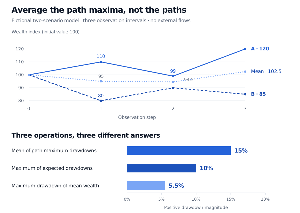
On A, the deepest decline is from 110 to 99: 10%. On B, it is from the initial 100 to 80: 20%. Include initial wealth in the running peak; otherwise B's first loss disappears from the calculation.
The expected maximum drawdown is therefore
0.5(10%)+0.5(20%)=15%.
No path in this model has a 15% maximum drawdown. That number is an average across possible outcomes. Half the probability lies at a drawdown greater than the average, so 15% is neither a loss ceiling nor a high-confidence risk limit.
Two equally likely fictional wealth paths have maximum drawdowns 10% and 20%, giving expected maximum drawdown 15%. Maximum expected pointwise drawdown is 10%; maximum drawdown of the mean wealth path is 5.5%.
Original fictional two-scenario model, initial wealth 100, three observation intervals and no external flows. Lines join observed values only. Average each path's maximum to obtain 15%; averaging earlier in the calculation changes the question.
Where the expectation belongs
Use positive fractional loss magnitudes throughout. For a random wealth path W0,…,WT, define its running peak, drawdown and maximum drawdown by
Ht=0≤s≤tmaxWs,Dt=1−HtWt,MT=0≤t≤TmaxDt.
Here T counts observation intervals, Wt>0, and the peak resets at time zero. The expected maximum drawdown is
EP[MT]=EP[0≤t≤TmaxDt].
The probability law P describes the possible paths and their weights. For a forecast of investment risk it should represent the intended real-world scenario assumptions. Risk-neutral pricing probabilities answer a different expectation and need explicit labelling.
Two tempting shortcuts produce different objects:
Take the maximum after averaging drawdowns at each date. In the example, expected drawdowns at steps 0–3 are 0%, 10%, 10% and 7.5%. Their maximum is 10%. A's worst loss arrives at step 2; B's arrives at step 1. Averaging date by date misses this scenario-specific timing. In general, maxtE[Dt]≤E[maxtDt], because each Dt is bounded above by the path maximum.
Average wealth first, then calculate its maximum drawdown. The mean path falls from 100 to 94.5 before recovering, giving 5.5%. This is the maximum drawdown of a deterministic mean curve. The curve is neither A nor B, and its running peaks differ from theirs. It does not measure the average worst loss experienced across the scenarios.
The order is the definition: path → running peak → worst fractional loss → average across paths.
What an estimate must hold fixed
For N independent, equally weighted paths generated from the chosen law, a Monte Carlo estimator is
E[MT]=N1i=1∑NMT(i).
More simulated paths reduce sampling error around that model's expectation. They do not repair missing crises, incorrect dependence, unrealistic execution or a valuation grid that misses intraperiod losses. Report Monte Carlo standard error separately from model uncertainty; overlapping historical windows are not independent simulation draws.
Horizon and monitoring. Extending the horizon of the same process, with its original starting peak retained, cannot reduce its path maximum or its expectation. Adding observation times to a nested grid also cannot reduce the measured maximum when values at shared times agree. A rolling-window reset is a different calculation. There is no universal annualisation multiplier: Magdon-Ismail and coauthors show that even absolute Brownian drawdown has different long-horizon growth rates depending on drift. Their absolute-loss formulas are not percentage-wealth formulas.
Path law and accounting. State the return model or resampling design, dependence assumptions, fees, financing, rebalancing and treatment of cash flows. Shuffling individual returns can erase loss clusters. Drawdown of a unitised investment index also differs from drawdown of an account balance affected by withdrawals. This percentage definition requires positive wealth; a strategy that can reach zero or negative equity needs an explicit failure convention.
For the accounting and historical measurement underneath a scenario study, Backtest Evaluation develops flow-adjusted wealth, drawdown recovery and resampling caveats. The full lesson requires membership, with a public preview.
Average worst loss and tail worst loss
Expected maximum drawdown averages all path maxima with their probabilities. Conditional expected drawdown instead takes a tail mean of the maximum-drawdown distribution at a specified confidence level. In this model, the worst half consists entirely of B, so its tail mean is 20%, compared with the unconditional mean of 15%. With discrete probability masses, define the tail using quantiles and the appropriate probability weight rather than relying on an ambiguous strict-threshold average. Goldberg and Mahmoud's definition makes this distinction precise.
Neither measure is automatically value at risk or expected shortfall of terminal portfolio loss. Those calculations concern a different random variable: an endpoint loss can conceal a severe interim decline and recovery.