An efficient estimator attains a precision benchmark within a stated model and class. Compare two unbiased return means and distinguish exact from asymptotic efficiency.
Efficient estimator
An efficient estimator reaches a precision benchmark within a specified statistical model and class of estimators. In the standard finite-sample sense, it is an unbiased estimator whose variance attains the Cramér–Rao lower bound when that bound applies.
The qualifications matter. “Efficient” does not mean fastest to compute, closest to the truth in every sample, or best under every measure of error. It describes how much repeated-sample uncertainty remains after the model, target and comparison rule have been fixed.
Two ways to average the same four returns
A researcher wants the unknown common mean μ of a strategy's one-period returns. For this illustration, stipulate four independent, identically distributed normal observations with known population standard deviation σ=2 percentage points (pp). These are model assumptions, rather than claims about actual strategy returns.
Compare the ordinary mean with a predetermined unequal-weight mean:
Both sets of weights sum to one, so both estimators have expectation μ. Neither systematically overshoots or undershoots the target. Their variances, however, differ:
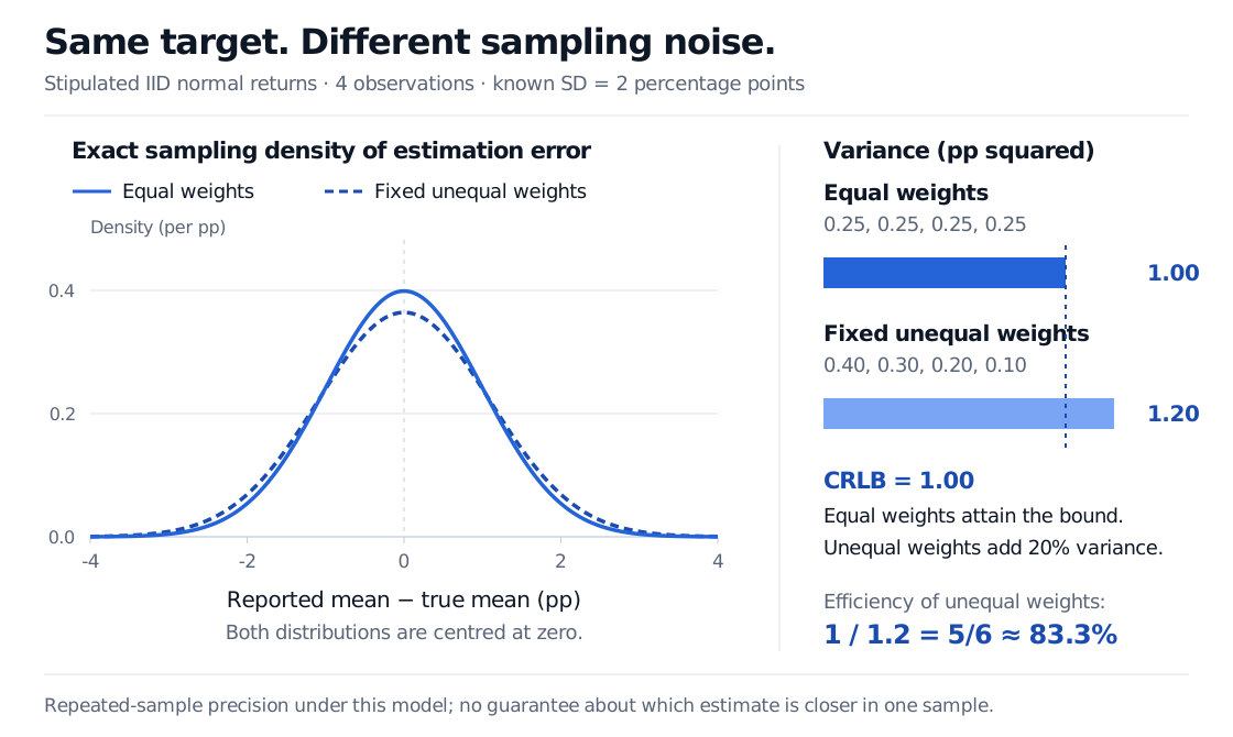
The unequal weights add 20% variance without reducing bias. In this model every observation is equally informative about the same mean, so giving one observation extra influence wastes precision.
This is visible directly. For any predetermined weights summing to one,
i=1∑nwi2=n1+i=1∑n(wi−n1)2≥n1.
With independent observations of equal variance, equal weights therefore minimise variance among these linear unbiased averages. That algebra does not require normality. The normal assumption lets us make the stronger claim below about all unbiased estimators of the mean.
Exact normal error densities for two unbiased means: equal weights have variance 1 pp squared; fixed unequal weights have variance 1.2 pp squared. Both are centred at zero. The CRLB is 1 pp squared, attained by equal weights.
Original stipulated IID normal model, not market data. Curves show exact sampling distributions of estimation error; bars show variance. The bound concerns unbiased estimators of the common mean.
Certifying that the mean reaches the limit
For a regular scalar-parameter model, let In(θ) be the full sample's Fisher information. Under the conditions needed for the Cramér–Rao inequality, an unbiased estimator θ^ with finite variance satisfies
Varθ(θ^)≥In(θ)1.
The conditions include sufficient differentiability and valid interchange of differentiation and integration in the relevant expectations; a parameter-dependent support needs particular care. Writing down a likelihood alone does not establish them.
In our normal location model, In(μ)=n/σ2. Thus the four observations supply information of 1pp−2 and the lower bound is 1pp2. The ordinary mean attains it for every real μ. It is exactly efficient at this sample size, not merely better than the one competitor we tried.
To quantify the unequal-weight estimator's shortfall, define its efficiency relative to the efficient mean as benchmark variance divided by candidate variance:
eff(T;Xˉ)=Var(T)Var(Xˉ)=1.21=65≈83.3%.
Always check which way a relative-efficiency ratio is defined. Here 100% means matching the benchmark. The 83.3% figure is a variance ratio, not a probability that the estimate is correct.
A lower bound need not be attainable. When no unbiased estimator reaches the Cramér–Rao number, an estimator can still have minimum variance among unbiased estimators without being CRLB-efficient. Conversely, attaining this bound does not certify optimality once biased estimators are admitted: mean squared error adds squared bias to variance, changing the comparison.
When “efficient” means large-sample efficient
Asymptotic efficiency concerns a sequence of estimators as sample size grows. In a regular IID scalar model, the usual information benchmark is
n(θ^n−θ)dN(0,I1(θ)1),
where I1(θ) is information from one observation. An asymptotically efficient regular estimator achieves this limiting distributional benchmark; the comparison is within the appropriate regular estimator class. Suitable maximum likelihood estimators have this property under the required model and regularity conditions. They need not be unbiased or CRLB-efficient at any particular finite sample size.
For a return forecast, the model remains the deciding qualification. Serial dependence changes the variance calculation. Unequal observation variances can make unequal weights useful. A changing mean can make recency weighting target something different from a fixed common mean. An efficiency result under the IID normal model does not settle those choices, nor does it guarantee a better trading decision from one realised dataset.
For the mathematical mechanism, the Cauchy–Schwarz derivation of the bound develops the score-covariance argument step by step (public preview; full lesson requires membership).
Sources
John A. Rice, Mathematical Statistics and Data Analysis, 3rd edition, §8.7, pp. 298–302.
George Casella and Roger L. Berger, Statistical Inference, 2nd edition, §7.3.2, Theorem 7.3.9 and Corollary 7.3.10.
UC Berkeley, STAT 135, Efficiency and Mean Squared Error, especially the distinction between finite-sample efficiency, asymptotic efficiency and sensitivity to assumptions.