A denoising autoencoder is an autoencoder trained to reconstruct an original observation from a deliberately corrupted version of it. For a quant researcher, this creates a way to learn features from unlabelled market snapshots while asking the network to cope with damaged inputs. It does not establish that the reconstructed prices are economically correct.
Keep the original; damage the input
Save an observation , sample a corrupted version from a chosen distribution , then pass the corrupted version through an encoder and decoder:
The loss function compares with the saved original . With summed squared error across coordinates, training minimises
This averages over training observations and their random corruptions. Masking selected coordinates or adding noise supplies different reconstruction tasks. The original paper used random zero masking; the target was still the uncorrupted example. See Vincent et al., Sections 2.2–2.4.
It is a form of self-supervised learning: targets come from available training observations, without requiring separately annotated outcomes. The hope is that recovering missing information teaches useful dependencies rather than a copying shortcut.
A target error of 0.08
Take a fictional, dimensionless observation . Mask its first coordinate, producing . Stipulate, rather than fit, the network reconstruction .
The correct summed squared reconstruction error is
Comparing the reconstruction with the corrupted input would instead give
That changes the learning task: it rewards reproducing the damage. Under the per-coordinate mean squared error convention, divide each sum by two: the values become and . Neither convention changes which target is correct.
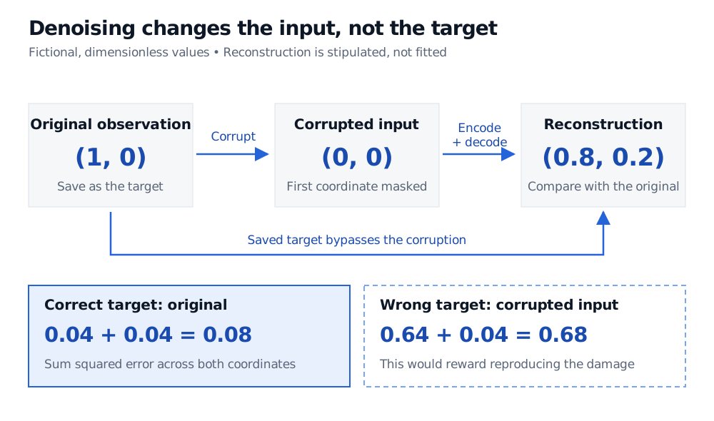
Original illustrative training pair, not a fitted model. Corruption changes the network input; the saved original remains the reconstruction target.
What “clean” can mean
“Clean” means before the added training corruption. A recorded market snapshot can already contain bid–ask effects, stale quotes or measurement error. Reconstructing it does not recover an independently observed, noise-free economic latent state.
There is also irreducible ambiguity. Under a population joint distribution of original and corrupted observations, finite second moments, unrestricted reconstruction functions and exact minimisation of expected squared error, the optimal reconstruction is the conditional expectation
Several originals can produce the same damaged input, so this conditional average need not equal any particular original. A finite fitted network need not attain that population optimum. Deep Learning, Section 14.5 develops the denoising objective and its reconstruction interpretation.
The corruption distribution is therefore a modelling choice: training on small independent perturbations does not certify robustness to a market regime change. Masking a genuine zero also leaves its missingness ambiguous unless the input design supplies that information.
Different regularisers, and a clock
A contractive autoencoder explicitly penalises the encoder's input Jacobian. A sparse autoencoder penalises code activations to encourage sparsity. Denoising instead changes the input–target pairing. These mechanisms can be combined, but their objectives are distinct; see Deep Learning, Sections 14.2 and 14.7.
For a historical forecasting experiment, fit scaling and the autoencoder only on observations eligible at the fitting date. Select corruption strength and architecture using a suitable validation period, then evaluate the downstream task on later held-out data. Pretraining on future market observations can introduce look-ahead bias even without return labels. Learned preprocessing must respect the same fitting boundary, as explained in scikit-learn's data-leakage guidance. Lower reconstruction error alone is not evidence of a better forecast.
For the underlying architecture, Autoencoders and Representation Learning Through Reconstruction has a public preview; the full lesson requires membership.
Sources
- Vincent, Larochelle, Bengio and Manzagol (2008), Extracting and Composing Robust Features with Denoising Autoencoders, Sections 2.2–2.4: original reconstruction target, stochastic corruption and representation learning.
- Goodfellow, Bengio and Courville, Deep Learning, Chapter 14, Sections 14.2, 14.5 and 14.7: denoising, conditional reconstruction and neighbouring regularisers.
- scikit-learn, Common pitfalls, Section 12.2: separation of training, model selection and held-out preprocessing.