An autoencoder with a sparsity constraint on its code activations. A worked Bernoulli KL penalty shows what a low mean activation does—and does not—guarantee.
Sparse autoencoder
A sparse autoencoder is an autoencoder trained to reconstruct its input while encouraging most code activations to be small or zero. In quantitative research, it offers a way to learn selective responses to market observations without requiring the code to have fewer coordinates than the input. Sparse activations do not automatically identify economically meaningful factors. The defining constraint acts on the representation, rather than requiring a narrow bottleneck. Deep Learning, Section 14.2.1 describes this reconstruction-plus-sparsity objective.
What is sparse?
An encoder produces a code h=fθ(x); a decoder reconstructs x^=gϕ(h). A sparse code uses relatively few substantial responses for an observation, or keeps each unit's response small on average, depending on the chosen penalty. The encoder and decoder can still have dense weight matrices. This is different from pruning connections or imposing zeros on weights.
One classical construction uses sigmoid code activations between zero and one. For hidden unit j, average its activation across m training observations:
ρ^j=m1i=1∑mhj(x(i)).
Choose a small target ρ and penalise deviations of each unit's average from that target. Ng's lecture notes, Section 3 use the Bernoulli Kullback–Leibler penalty:
Here k is the number of code units and β>0 sets the sparsity penalty's weight. Natural logarithms give the KL term in nats. The penalty is nonnegative and is zero when ρ^j=ρ; it also penalises a mean below the target. This is a preference for a particular low mean, not a command to push every activation to zero.
Read the penalty before interpreting the code
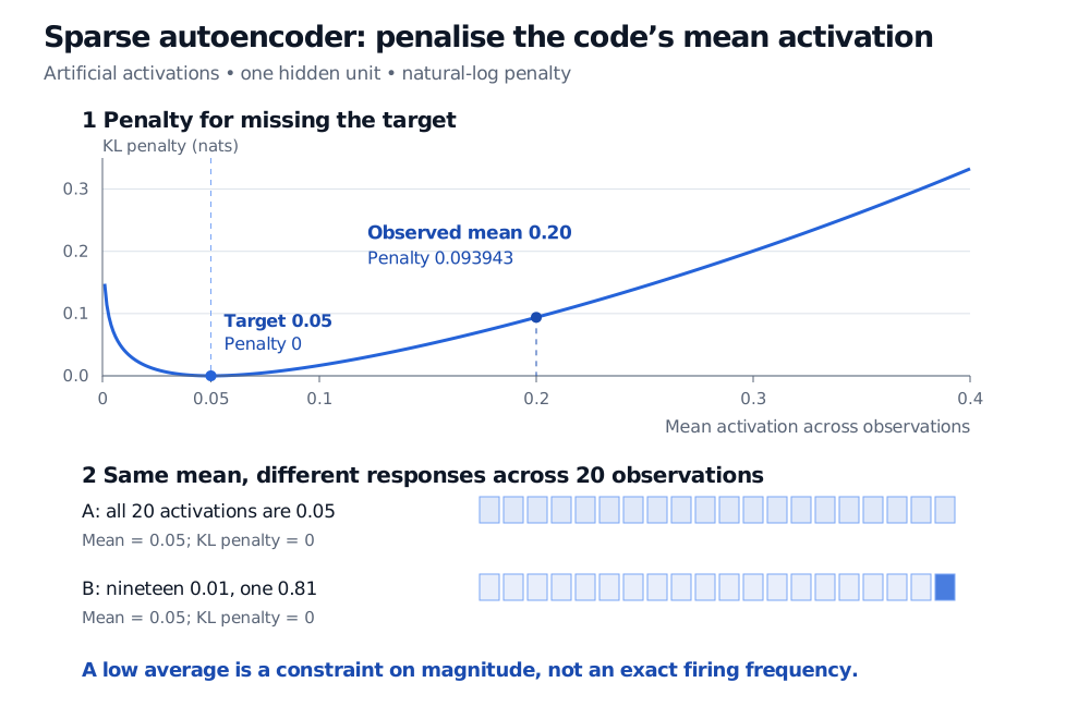
Take one unit with target ρ=0.05 and observed mean ρ^j=0.20. Its unweighted contribution is
0.05ln0.200.05+0.95ln0.800.95=0.093943026….
This is one unit's KL penalty, before multiplication by β and summation over units. It is neither a reconstruction error nor a forecast score.
A target mean of 0.05 does not say that a unit fires on exactly 5% of observations. Consider two artificial profiles across 20 observations. In profile A, every activation is 0.05. In profile B, nineteen activations are 0.01 and one is 0.81. Both means equal 0.05, so both receive zero mean-activation KL penalty. Their responses are quite different: with an illustrative firing threshold of 0.5, A never fires and B fires once. The mean penalty alone cannot distinguish them; reconstruction and the rest of the model still matter.
Artificial one-unit example: target mean activation 0.05 and observed mean 0.20 give Bernoulli KL penalty 0.093943 nats. Two 20-observation profiles both average 0.05: all values 0.05, or nineteen values 0.01 and one value 0.81.
Original illustrative activations, not a fitted model. The penalty is zero at the target mean, but that mean can arise from very different response patterns.
Choose the constraint to match the activation
The Bernoulli construction above needs probability-like activation values and a mean strictly between zero and one; it cannot be applied unchanged to unbounded ReLU outputs. An alternative penalises the code's absolute values, often called an L1 activation penalty. ReLU codes can also contain exact zeros, whereas finite sigmoid outputs are merely close to zero. These choices create different objectives; “sparse autoencoder” does not specify a single penalty or activation function. Deep Learning, Section 14.2.1 discusses absolute-value penalties and rectified codes. A denoising autoencoder instead learns from deliberately corrupted inputs; the two ideas can be combined.
For an illustrative market-state feature pipeline, fit scaling and the encoder on the training period, then evaluate the frozen transformation on later observations. Check activation distributions as well as reconstruction and the actual downstream task. A sparse representation with low reconstruction loss is not evidence of return predictability, causal structure or stable “true” economic factors. Those are separate claims requiring separate evidence.