Removing neural-network weights or channels: magnitude masks, structured pruning, fine-tuning and why sparsity alone does not establish faster inference.
Neural network pruning
Neural network pruning removes selected weights or larger structures from a neural network, usually to reduce the resources needed to store or run it. For a quant model serving forecasts repeatedly, pruning can be a compression experiment—but fewer nonzero weights do not by themselves establish faster predictions or preserved forecast quality.
The key decisions are what to remove, how to recover the fit, and whether the deployed system can exploit the removal.
A mask is a decision about connections
A common starting point is magnitude pruning: rank trained weights by their absolute values and remove the smallest. For weights wi and a binary keep mask mi, the effective weights are
wi=miwi,mi∈{0,1}.
Consider four illustrative trained weights, in their original order:
w=(0.10,−0.02,0.80,−0.60).
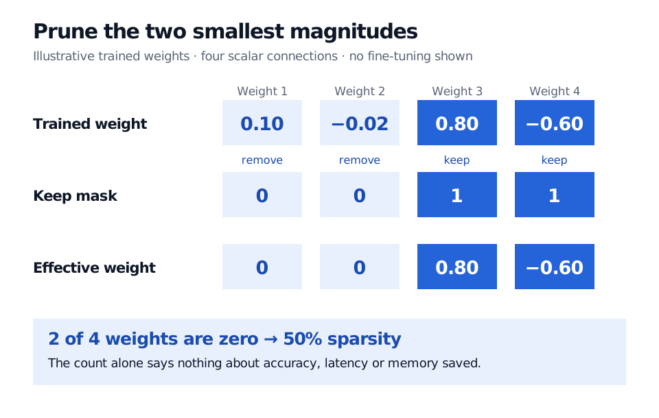
Pruning the two smallest magnitudes removes −0.02 and 0.10, so
m=(0,0,1,1),w=(0,0,0.80,−0.60).
The negative weight −0.60 survives because its magnitude is large. Counting zeros among these four selected scalar weights gives
sparsity=number of weightsnumber of zero weights=42=50%.
This is a parameter-count result, with no accuracy or timing measurement. A whole-model sparsity figure must also say which tensors are included: pruning one layer does not make every layer equally sparse.
Four trained weights 0.10, −0.02, 0.80 and −0.60 become effective weights 0, 0, 0.80 and −0.60 under mask 0, 0, 1, 1; two of four zeros give 50% sparsity.
Illustrative magnitude pruning: remove two individual connections, preserving their original coordinate positions. Fifty per cent sparsity is not a performance benchmark.
Magnitude is a heuristic for importance. A small coefficient multiplying a large activation may still matter. Rescaling adjacent layers can change weight magnitudes while preserving the network's function, so a magnitude ranking depends on the model's parametrisation. Compare the resulting predictions and loss; the ranking alone cannot prove that a connection is dispensable.
Individual zeros versus a smaller layer
Approach
Removal unit
Consequence for execution
Unstructured pruning
Individual scalar weights, as above
Produces an irregular pattern of zeros; acceleration requires suitable sparse storage and execution.
Structured pruning
Whole units, filters or channels
Can reduce tensor dimensions when the model is rebuilt consistently, allowing smaller dense operations.
For a convolutional channel, physical removal includes its producing filter and the corresponding inputs in the next layer. Dependencies such as residual additions must remain compatible. Merely masking a whole channel while leaving the same tensor shapes is not the same as rebuilding a narrower network. Li et al. develop filter pruning around this distinction.
A dense matrix kernel may perform the same work on zero entries as on nonzero ones. Sparse formats also need indices, and real latency depends on hardware, batch size and the operations around the pruned layer. Measure the exported model in its intended setting rather than translating sparsity directly into a speedup.
Prune, recover, then evaluate
Han et al. describe training a dense network, pruning connections and retraining the survivors. Fine-tuning lets the retained weights adjust to the changed computation; it does not guarantee recovery. Pruning and recovery can also be repeated in stages.
For financial data, fit the initial model, compute data-dependent importance scores and fine-tune using training observations only. Use a separate chronological validation period to choose the pruning amount and recovery settings. Reserve an untouched later test period for the final comparison. Trying many masks against that test period makes pruning another route to overfitting.
Keep the mask enforced during recovery. Zeroing a parameter once does not prevent later updates from making it nonzero: gradients and stored optimiser momentum can move it again. After physically changing tensor shapes, rebuild or deliberately migrate the optimiser state so it matches the surviving parameters.
The current PyTorch pruning tutorial illustrates a masked representation using an original weight tensor plus a mask. Removing that pruning reparametrisation keeps the current zeros but removes the masking mechanism; subsequent unconstrained training can regrow them. A masked training checkpoint can retain both original weights and masks, so its size is not evidence of compressed deployment storage.
Pruning also differs from dropout, which normally samples temporary omissions during training. The lottery ticket hypothesis asks a separate question about training selected subnetworks from particular initialisations; finding a sparse trained model does not establish that hypothesis.
For the surrounding model-selection discipline, SelfMadeQuant's regularisation and validation lesson compares weight decay, dropout and early stopping with a held-out selection protocol. The preview is public; the full lesson requires membership.
Li, Kadav, Durdanovic, Samet and Graf (2017), Pruning Filters for Efficient ConvNets, §§1 and 3: structured filter removal and its computational motivation.
PyTorch, Pruning Tutorial, “Pruning a Module,” “Serializing a pruned model” and “Remove pruning re-parametrization”; checked 1 November 2026.