Contractive autoencoder: Definition & Examples

A contractive autoencoder is an autoencoder trained with a penalty on how sensitive its encoder is to small input changes. In quantitative research, this offers a way to discourage unstable features extracted from noisy market snapshots. Whether those features improve a forecast must still be tested on later, unseen data.

What contracts?

Write the encoder as $h=f_\theta(x)$ and the decoder as $\hat x=g_\phi(h)$ . A common training objective is

\frac{1}{n}\sum_{k=1}^{n}\left[ L\left(x_k,g_\phi(f_\theta(x_k))\right) +\lambda\lVert J_f(x_k)\rVert_F^2 \right],\qquad \lambda\ge 0,

where $L$ measures reconstruction error. The Jacobian matrix $J_f$ contains the derivatives of the encoded features with respect to the inputs:

\lVert J_f(x)\rVert_F^2 =\sum_{j=1}^{d_h}\sum_{i=1}^{d_x} \left(\frac{\partial h_j}{\partial x_i}\right)^2.

The reconstruction term asks the code to retain information; the penalty discourages rapid changes in that code. It penalises the encoder, not the decoder Jacobian or the Jacobian of the complete reconstruction map. This is the defining distinction in Rifai et al., Sections 2–4.

A penalty of 0.025, step by step

Consider a fixed scalar encoder on a dimensionless, scaled input:

h(x)=\sigma(2x),\qquad \sigma(u)=\frac{1}{1+e^{-u}}.

This is a calculation example, not a trained financial model. At $x=0$ ,

\begin{aligned} h(0)&=0.5,\\ h'(0)&=2h(0)(1-h(0))=0.5,\\ \lVert J_f(0)\rVert_F^2&=(0.5)^2=0.25,\\ \lambda\lVert J_f(0)\rVert_F^2&=0.1\times0.25=0.025. \end{aligned}

The coefficient

\lambda=0.1

is stipulated for this example. The 0.025 is only the contractive contribution, not total loss: a reconstruction value requires a specified decoder and reconstruction-loss convention.

For an input increase of $0.01$ , the local linear approximation predicts a code increase of $0.5\times0.01=0.005$ . Direct evaluation gives $h(0.01)-h(0)\approx0.00499983$ . The close agreement illustrates what the derivative measures near this point.

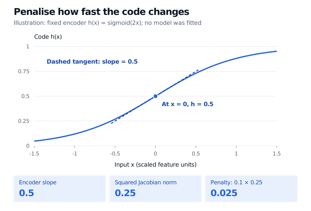
Fixed encoder h(x) = sigmoid(2x), not a fitted model: at x = 0 the code is 0.5 and tangent slope is 0.5. The squared encoder Jacobian norm is 0.25; coefficient 0.1 gives penalty 0.025.

The dashed tangent measures local encoder sensitivity. The three quantities below the chart are a derivative, its square and the weighted penalty; they are not reconstruction errors.

Stable features can still be useless

A constant encoder has zero input sensitivity. That makes it ideal for the penalty alone, yet it cannot distinguish different inputs for reconstruction. The two training terms must therefore be balanced. Architecture matters too: the original paper used tied encoder–decoder weights, limiting a trivial strategy of shrinking the code and compensating with a more expansive decoder.

Small derivatives at training observations encourage local stability. They do not impose a global contraction bound, guarantee invariance to finite shocks, or certify protection against adversarial inputs. The geometric interpretation and its local scope are discussed in Deep Learning, Section 14.7.

Two neighbouring methods target different objects:

Method	Training pressure
Contractive autoencoder	Penalise derivatives of the encoder with respect to its inputs.
Denoising autoencoder	Reconstruct a clean target from a deliberately corrupted input.
Sparse autoencoder	Encourage sparse code activations; sparsity and low sensitivity are different properties.

These distinctions are set out in Deep Learning, Sections 14.2.1–14.2.3.

For market data, define feature scales before interpreting the penalty: changing from decimal returns to percentage units changes derivatives with respect to those coordinates. Fit scaling and encoder parameters using training data only. Choose the penalty strength on validation data under the intended time ordering, and assess the downstream task as well as reconstruction. Suppressing a feature's reaction to genuine market changes can remove useful information along with noise.

For the underlying architecture, see Autoencoders and Representation Learning Through Reconstruction (full lesson requires membership).

Sources

Rifai, Vincent, Muller, Glorot and Bengio (2011), Contractive Auto-Encoders: Explicit Invariance During Feature Extraction, Sections 2–4 and 5.3: original objective, sigmoid penalty and local contraction interpretation.
Goodfellow, Bengio and Courville, Deep Learning, Chapter 14, Sections 14.2.1–14.2.3 and 14.7: sparse, denoising and contractive objectives and their limitations.

What contracts?

A penalty of 0.025, step by step

Stable features can still be useless

Sources

Related terms

Denoising autoencoder

Sparse autoencoder