DeepAR learns conditional forecast distributions with one autoregressive recurrent network shared across related time series. Understand its likelihood, sampling and dependence limits.
DeepAR
DeepAR is a probabilistic forecasting method that trains one autoregressive recurrent neural network across many related time series. It predicts a distribution for the next observation, then samples recursively to produce future paths. For a quant forecasting activity across venues or instruments, the attraction is learning recurring patterns across series while retaining uncertainty about each future outcome. Sharing information helps only when the series contain transferable structure.
One shared network, many separate states
A recurrent neural network updates a state from the previous state, the latest target observation and available features. In schematic DeepAR notation,
Here i identifies the series, xi,t contains covariates, and θi,t contains the next-step distribution's parameters. The weights Θ are shared across series; the states hi,t differ. The original architecture uses LSTM cells. Training maximises conditional log-likelihood over observed windows. Salinas, Flunkert and Gasthaus, §3.
“Global” describes shared learning. It does not automatically supply a joint cross-series shock model. Independently sampling forecasts for two venues can miss simultaneous activity spikes even when their separate forecasts are good. Temporal dependence within a sampled path and dependence between different series are distinct requirements.
Amazon's DeepAR description explains learning across related series, including static categorical features and dynamic covariates. A short-history series may benefit from patterns learned elsewhere; a series unlike the training population may not.
The output is a distribution, not just its mean
The distribution family is chosen by the modeller; the network outputs its conditional parameters. The original paper's experiments use Gaussian likelihoods for real-valued observations and negative binomial distributions for counts. Positive parameters are constrained to remain valid. DeepAR, §3.1.
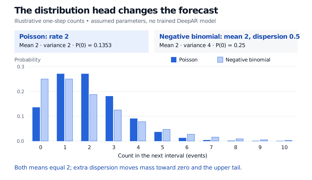
For a deliberately simpler illustration, suppose a possible count head outputs a Poisson rate of λ=2 events for the next interval. This is an assumed conditional distribution, not a trained DeepAR result or the original paper's count choice. Its probability mass is
P(Y=k∣available history)=e−2k!2k,k=0,1,2,…
The probability of no events is e−2≈0.1353353, or about 13.53%. The conditional mean is 2 events and variance is 2 events squared. “Predicts 2” discards the distinction between a likely outcome and an average over possible outcomes.
For comparison, a negative binomial head with mean μ=2 and dispersion α=0.5, using the paper's parameterisation, has variance μ+αμ2=4 and zero probability (1+αμ)−1/α=0.25. The same mean can accompany more zeros and a heavier upper tail. Choosing a head whose variance must equal its mean can understate count uncertainty when conditional overdispersion remains.
Illustrative one-step count distributions: Poisson rate 2 has mean 2, variance 2 and probability of zero 0.1353. Negative binomial mean 2 and dispersion 0.5 has variance 4 and probability of zero 0.25. Bars show counts from 0 to 10; remaining upper-tail mass is omitted.
Original assumed-parameter comparison, not fitted forecasts. The Poisson head is a pedagogic possibility; the original DeepAR paper uses a negative binomial likelihood for count experiments. Both distributions extend beyond the plotted counts.
A future path must feed back its own draws
At prediction time, first run through the observed context. Draw the first future value from its conditional distribution, feed that draw back into the recurrent update, and continue. Repeat the whole procedure for many paths. This is autoregressive generation; replacing draws with conditional means generally changes the resulting path distribution. DeepAR, §3 and Figure 2.
For a multi-interval activity total, sum within each sampled path before estimating its quantiles. Adding separate interval quantiles generally does not give the total's quantile. Shuffling draws independently across dates also destroys the temporal dependence that recursive sampling was designed to preserve.
Information and scale still constrain the forecast
Calendar features are known ahead of time. Tomorrow's realised market volume is not. Dynamic predictors required over the horizon must be available at the forecast origin, supplied as explicit scenarios, or forecast separately. Treating a scenario as certain omits uncertainty about that scenario. Amazon's algorithm guide makes the known-future feature requirement explicit.
Scale also matters when one venue has far more events than another. DeepAR uses series-specific input scaling and corresponding likelihood-parameter adjustments; scaled count inputs do not turn the observed integer target into a continuous response. Estimate preprocessing from information available at the origin to avoid look-ahead bias. The paper discusses scaling in §3.3.
Evaluate later forecast origins against sensible benchmarks, checking distributional coverage and tail behaviour as well as point errors. A fitted likelihood does not ensure calibrated prediction intervals, resilience to market changes or economic value.
The SelfMadeQuant lessons Recurrent Networks for Structured Data and Forecast Evaluation develop the recurrent-state mechanism and chronological evaluation design. Both have public previews; their full lessons require membership.