A generative model that builds a joint distribution from ordered conditional distributions, illustrated by a two-bit probability tree and the distinction between training and sampling.
Autoregressive generative model
An autoregressive generative model represents a joint probability distribution as an ordered product of conditional distributions, then generates a new observation by sampling one component after another. For a quant building synthetic return sequences or order-event scenarios, the crucial consequence is that each new draw can depend on the scenario already generated. A collection of individually plausible draws need not have the right dependence.
A distribution built from prefixes
Choose an ordering of the components x1,…,xT. The probability chain rule gives
pθ(x1,…,xT)=t=1∏Tpθ(xt∣x<t),
where x<t denotes earlier components and θ the model parameters. At the first position, the prefix is empty. For discrete variables these factors are probability masses; for continuous variables they are conditional densities.
The identity itself is exact. The modelling choices are how to parameterise the conditional probabilities, which preceding components the network can use, and how well those distributions are learned. Normalised conditionals yield a normalised joint distribution. Restricting a network's receptive field can limit the dependence it captures even though its output remains a valid probability law.
“Earlier” need not mean earlier in calendar time. PixelCNN orders image pixels and colour channels, using masked convolutions to prevent access to components that have not yet been generated. A fixed image thereby becomes a sequence-modelling problem. The original PixelRNN/PixelCNN paper, §§2.1 and 3.4–3.5, describes this ordering and masking.
WaveNet instead generates waveform samples in temporal order using causal, dilated convolutions. Dilation expands the receptive field without allowing future audio samples into a prediction. WaveNet, §§2–2.1.
This is broader than a linear autoregressive time-series model, which specifies a linear relationship between a series and its lags, together with innovations. Such a process can be used generatively once its initial and innovation distributions are specified. Neural autoregressive generation does not require linearity, stationarity or a time-series interpretation.
Two bits, four complete scenarios
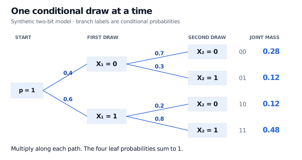
Consider a synthetic two-bit sequence. Let X1 equal 1 with probability 0.6. Let X2 equal 1 with probability 0.8 after X1=1, but only 0.3 after X1=0.
Sequence
Product along the path
Joint probability
00
0.4×0.7
0.28
01
0.4×0.3
0.12
10
0.6×0.2
0.12
11
0.6×0.8
0.48
The probabilities sum to one. Sequential sampling first draws X1, then uses the conditional distribution appropriate to that realised bit to draw X2. Repetition follows exactly this law.
Synthetic probability tree: the first bit is 1 with probability 0.6. The second bit is 1 with probability 0.3 after 0 and 0.8 after 1. Joint masses for 00, 01, 10 and 11 are 0.28, 0.12, 0.12 and 0.48.
Original synthetic two-bit example. A branch probability is conditional; a leaf probability is the product along its path. No fitted financial data are used.
The second bit's unconditional probability of 1 is also 0.6: the two relevant leaves have masses 0.12+0.48. Drawing both bits independently with probability 0.6 would instead assign probability 0.36 to 11. Matching the two marginals has lost the dependence.
Always choosing the more probable next bit produces only 11 here. That is greedy decoding, not sampling from the table. More generally, altering conditional probabilities during decoding changes the generated law.
Observed prefixes for training, generated prefixes for sampling
Under ordinary teacher forcing, the model scores the actual next component using the actual preceding components in a training observation. Maximum likelihood maximises the sum of these conditional log-probabilities. For the observed sequence 11 in the example, the negative log-likelihood is
−ln(0.6)−ln(0.8)=−ln(0.48)≈0.73397 nats.
All prefixes of an observed sequence are available. Masked or causal convolutional architectures can therefore score positions in parallel during training. Ordinary ancestral generation must wait for earlier samples, then feed them back as context. WaveNet explicitly distinguishes these two computations in §2.1.
A causal language model uses the same next-component idea with tokens; Hugging Face's current guide describes restricting attention to preceding tokens. “Causal” here means respecting the generation order, not identifying an economic cause.
At generation time, an imperfect model may visit prefixes uncommon in its training data. Subsequent errors can then accumulate, the training/inference mismatch described by Bengio et al. (2015). Teacher forcing is nevertheless a valid way to evaluate the joint likelihood; it does not mathematically invalidate the factorisation.
For financial scenarios, evaluate full generated paths and their dependence, tail behaviour and stability across market conditions. A good conditional likelihood on held-out observations is useful evidence, but it does not by itself establish realistic long rollouts. Generation order also cannot repair future information leaking into training features.
For the probability mechanics behind the tree, Probability Fundamentals develops conditioning and independence; the full lesson requires a free account.