Compute an oriented 3D cross product, interpret its length as area, and construct a fictional three-asset position that cancels two specified factor exposures.
Cross product
The cross product takes two vectors in oriented three-dimensional Euclidean space and returns a vector perpendicular to both. Its length is the area of the parallelogram spanned by the inputs; its direction follows the right-hand rule. Unlike the dot product, which returns a scalar, it produces a new vector.
For a quant, a useful small example is finding a three-asset position with zero exposure to two specified factors. The same construction also finds normals to planes. The operation is inherently tied to the usual oriented 3D geometry: it is not a general algorithm for hedging an arbitrary number of assets.
Compute the vector, then check its sign
In a right-handed orthonormal coordinate system, let a=(a1,a2,a3) and b=(b1,b2,b3). Then
a×b=(a2b3−a3b2,a3b1−a1b3,a1b2−a2b1).
The middle component is a frequent sign trap. Written as the negative of a minor, it is −(a1b3−a3b1), which equals the second component above. A determinant with unit vectors in its first row is a useful mnemonic, but the component formula is the actual definition.
If n=a×b, the perpendicularity checks are
a⋅n=0,b⋅n=0.
These checks alone cannot distinguish n from −n. Orientation supplies the choice. For nonparallel inputs, curl the fingers of your right hand from the first input toward the second, through the smaller angle; your thumb points along their cross product. Reversing the order reverses the answer:
b×a=−a×b.
For example, the coordinate unit vectors satisfy e1×e2=e3, rather than −e3.
A fictional two-factor hedge
Suppose three fictional assets have the following dimensionless return loadings. The columns are assets; the rows are two specified factors.
Loading
Asset 1
Asset 2
Asset 3
Factor A, a
1
1
0
Factor B, b
0
1
1
For this example, write each asset's return as ri=aifA+bifB+εi, where fA,fB are factor returns and εi is the remaining asset-specific return. If wi is the signed dollar position divided by a common reference capital amount, the portfolio's factor coefficients are a⋅w and b⋅w. The target is to set both to zero.
Take the cross product of the loading rows, each viewed as a vector across the three assets:
Both exposures vanish: 1−1+0=0 for Factor A and 0−1+1=0 for Factor B. There is also a direct way to verify the construction. The constraints say w1+w2=0 and w2+w3=0, so every solution is w=t(1,−1,1) for a scalar t.
The cross product has selected a direction, not an investment size. For gross exposure of one unit of reference capital, divide by the sum of absolute components:
w=3(1,−1,1)=(31,−31,31),i=1∑3∣wi∣=1.
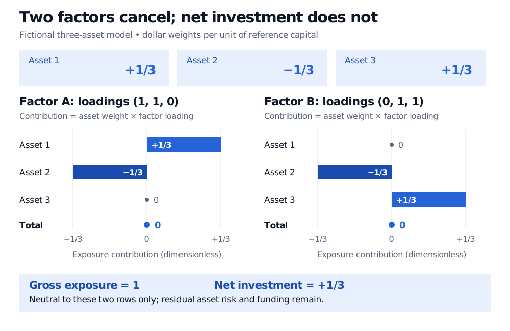
This means long one-third in Asset 1, short one-third in Asset 2, and long one-third in Asset 3. Long exposure totals two-thirds and short exposure one-third. Net investment is therefore positive one-third, not zero. Dividing instead by the Euclidean norm would give a unit-length vector, which is a different size convention.
Fictional three-asset weights one-third, negative one-third, one-third cancel two loading rows. Factor A contributions are one-third, negative one-third, zero; Factor B contributions are zero, negative one-third, one-third. Both totals are zero, while net investment is positive one-third.
Original fictional factor-exposure diagram. Weights are signed dollar positions per unit of reference capital; the loading rows and contributions are dimensionless. Gross exposure is one; net investment is positive one-third.
Only the two specified common-factor terms cancel. The residual ∑iwiεi remains, as do risks from omitted factors, changing loadings, trading costs and financing. This construction does not imply a riskless position, mean reversion or an arbitrage. Reversing the factor order gives the opposite trade with the same two zero exposures.
Length measures area, not portfolio risk
For nonzero inputs with angle θ∈[0,π],
∥a×b∥=∥a∥∥b∥sinθ.
This is base times perpendicular height: the parallelogram area. A triangle with the same two edge vectors has half that area. Here, ∥a∥=∥b∥=2 and a⋅b=1, so cosθ=1/2 and θ=60∘. Thus the cross-product length and parallelogram area are 3, while the triangle area is 3/2. These are geometric quantities in loading-coordinate space, not measures of portfolio variance.
An independent algebraic check is
∥a×b∥2=∥a∥2∥b∥2−(a⋅b)2=2⋅2−12=3.
If the inputs are parallel, or either is zero, the cross product is zero. For example, (1,1,0)×(2,2,0)=(0,0,0). There is then no cross-product direction to normalise. In the hedge interpretation, two nonzero proportional loading rows impose only one independent constraint, leaving a plane of possible three-asset positions rather than one line. If both rows are zero, neither constrains the position. Nearly proportional rows can also make the inferred direction sensitive to small estimation errors.
For more assets or additional constraints, formulate the exposure matrix and solve for its null space. In this example, adding a zero-net-investment constraint would require w1+w2+w3=0. Since the two factor constraints already force (w1,w2,w3)=(t,−t,t), the extra condition forces t=0. No nonzero position satisfies all three constraints with these loadings.
Steven G. Krantz and Harold Parks, Vector Calculus, first edition, CRC Press, 2024, §1.4, especially Definition 1.4.1, Theorem 1.4.2 and §§1.4.2–1.4.3.