Infer a proportional bid–ask spread from one-day and two-day high–low ranges, with explicit overnight adjustment, pair timing and negative-estimate conventions.
Corwin–Schultz spread estimator
The Corwin–Schultz spread estimator infers a proportional bid–ask spread from the high and low transaction prices of two consecutive trading days. Its practical attraction is historical coverage: researchers can construct a spread proxy when daily price ranges survive but intraday trades and quotes do not. It does not observe the spread available to an order at a particular instant.
The identification idea compares two separate one-day ranges with one combined two-day range. Under the model, efficient-price variance scales with the interval's length, while a constant spread enters each observed range. That distinction lets the estimator separate two contributors to the same high–low data. Corwin and Schultz's original paper, §1, develops the argument; the final article appeared in the Journal of Finance in 2012.
One pair, three range measurements
Let Ht,Lt be the positive high and low on trading day t. First consider a pair requiring no overnight adjustment. Define
Use natural logarithms. The two terms in βt are summed, not averaged. The two-day high is the larger daily high; the two-day low is the smaller daily low. Neither is an average price.
The last equality provides a convenient numerical evaluation. St is a full proportional spread in decimal units: 0.02 means 2%, or 200 basis points. It is not a dollar spread or an annualised statistic. A half-spread cost would be half this value under the symmetric model, before other trading costs.
The pair labelled t uses day t+1's completed range. It becomes available only after that session ends. A backtest that uses it to trade on day t introduces look-ahead bias.
Identical daily ranges: an exact arithmetic check
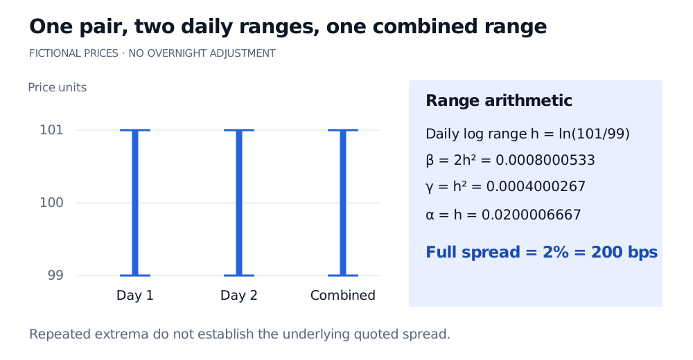
Take two fictional days, each with high 101 and low 99. Assume the preceding close lies inside the next day's range, so the overnight rule below does nothing. Put h=ln(101/99)=0.0200006667. Then
βt=2h2=0.0008000533,γt=h2=0.0004000267.
Consequently αt=h and
St=2101/99+1101/99−1=0.02=2%.
Fictional days 1 and 2 both have high 101 and low 99 price units. The combined range is still 99 to 101. The sum of squared daily log ranges is 0.0008000533, twice the combined squared range 0.0004000267; the estimated full spread is 2%, or 200 bps.
Original fictional example, with no overnight adjustment needed. Daily extrema are ranges, not a path showing when highs and lows occurred.
This is an exact check of the formula on constructed inputs. Identical observed ranges do not establish that the real market's quotes were 99 and 101, or that its true spread was 2%.
Overnight moves require an explicit rule
A move while the market is closed can enlarge the combined range without entering either intraday range. Holding βt fixed, a larger γt lowers αt, potentially making the raw spread negative.
The authors' practical adjustment compares day t's close with day t+1's entire high–low range. If the next low exceeds the prior close, their original rule shifts both next-day extrema down by that price difference. If the next high is below the prior close, it shifts both up. If the prior close lies inside the next range, it makes no adjustment. Thus a prior close of 100 and next-day low/high of 105/107 gives adjusted extrema 100/102. This is a heuristic for the nonoverlapping part, not a measurement of every overnight return. It is not an unconditional close-to-open subtraction. The published Internet Appendix, Table IA.II, distinguishes these rules.
Implementation details matter here: the original description shifts price levels; the checked package-author implementation shifts log extrema for the combined range and retains unadjusted intraday log ranges in β. Those operations are not numerically identical. Record the convention used, maintain consistent corporate-action adjustments, and never mix a split-adjusted close with raw highs and lows.
Truncate each pair before averaging
Finite-sample ranges need not obey the model's expectation relationships. In the displayed formula, γt>βt gives a negative raw estimate. That is an estimation outcome, not a negative economic bid–ask spread.
For the authors' pairwise correction, replace each negative estimate by zero, then average the resulting values across the valid overlapping pairs in the reporting window:
Spairwise=N1t∈I∑max(St,0),N=∣I∣.
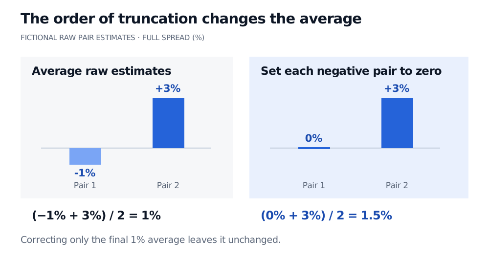
Corwin's March 2014 clarification stresses this order. It differs from retaining negative estimates, dropping those pairs, or correcting only the final average. For fictional raw pair estimates of −1% and +3%, pairwise truncation gives (0+3)/2=1.5%. Their raw average is 1%; truncating that average leaves 1%.
Fictional raw two-day spread estimates of minus 1% and plus 3% average to 1%. Setting each negative pair to zero first gives values 0% and 3%, averaging to 1.5%.
Original arithmetic comparison. Correcting each pair and correcting only the final average define different statistics.
Labels such as CS1 and CS2 need an accompanying formula. In the checked bidask source, CS2 truncates each pair before averaging; CS averages raw pair estimates and, when signed estimates are disabled, takes the absolute value of that average. It is therefore unsafe to assume that every unsuffixed CS or CS1 label means the authors' pairwise correction. Averaging β and γ before applying the nonlinear formula is another distinct construction.
State whether a monthly window includes only pairs fully inside the month, how missing sessions are treated, and how many valid pairs remain. Consecutive pairs share a day, so their estimates are not independent observations. A zero created by truncation does not establish costless execution.
What the range proxy leaves unresolved
The derivation assumes a diffusion for efficient value, a spread and variance constant over the pair, and highs at buyer-initiated prices and lows at seller-initiated prices. Its closed form also uses an approximation when converting range moments. It should not be described as an exact, universally unbiased recovery of spreads.
Sparse trading can miss the underlying extrema; stale or erroneous prints can distort them. Zero-volume days and days with high equal to low require an explicit data policy, rather than silent substitution. Jumps, rapidly changing volatility or spreads, and trading restrictions weaken the comparison of one-day and two-day ranges. The published appendix documents that data adjustments and negative raw estimates occurred in the authors' sample; their empirical results do not remove these issues for a new market.
The Parkinson volatility estimator instead treats the range as a variance signal. The Abdi–Ranaldo spread estimator uses closes relative to adjacent log midranges. These are different identification strategies, not interchangeable names for a daily spread statistic.
For quote-based measurement and the Roll covariance benchmark, the Spread Measurement lesson has a public preview; the full lesson requires membership. Whatever the estimator, a spread proxy alone does not describe order-book depth, fees or the market impact of a large order.