Estimate a proportional effective spread from daily log highs, lows and closes, with explicit adjacent-session indexing, negative-estimate correction and data-availability timing.
Abdi–Ranaldo spread estimator
The Abdi–Ranaldo spread estimator infers a proportional effective bid–ask spread from daily high, low and closing transaction prices. It is useful when a historical research dataset contains prices but no quotes: the close's position relative to two neighbouring daily midranges supplies a spread signal. It estimates a trading-cost proxy, rather than observing the bid–ask spread available for an order at a particular time.
Abdi and Ranaldo call the method CHL, for close, high and low. Their original paper, §1, gives the model and two ways to handle negative finite-sample estimates. Choosing between those versions is part of defining the statistic.
Two daily midranges around one close
For consecutive trading sessions t, let Ht, Lt and Ct be the positive high, low and close on a common price-adjustment basis. Use natural logarithms:
ht=lnHt,lt=lnLt,ct=lnCt,ηt=2ht+lt.
The midrange ηt is the average of log prices: equivalently, ηt=lnHtLt. It is neither ln((Ht+Lt)/2) nor a midquote assembled from bid and ask quotes.
Construct an adjacent-session product
xt=(ct−ηt)(ct−ηt+1).
Both factors use the same close ct. The second factor does not use ct+1. With complete data for sessions 1,…,N+1, there are N such products, indexed t=1,…,N. The final session supplies a midrange; its close is unused. For a calendar-month estimate, explicitly assign products by their close date t and retain the following session's high and low, even when it falls in the next month.
The monthly-corrected construction pools those products, then truncates the estimated squared spread before taking the square root:
smonth=max{N4t=1∑Nxt,0}.
The divisor is the number of valid products N. This is an uncentred sample moment, not a demeaned sample covariance with an N−1 divisor. If observations are missing, define the valid adjacent pairs and count those pairs; silently connecting across omitted sessions changes the construction.
The output is a full spread in decimal log-price units, approximately a proportional spread for small values. Multiplying by 104 gives an approximate basis-point quotation. It is not a dollar spread, a half-spread, or an annualised volatility; there is no square-root-of-time annualisation.
Three fictional sessions give two products
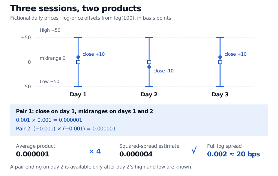
Suppose each session has Ht=100e0.005 and Lt=100e−0.005. The closes are 100e0.001, 100e−0.001 and 100e0.001.
Session
High
Low
Close
ct−ηt
1
100.501252
99.501248
100.100050
0.001
2
100.501252
99.501248
99.900050
−0.001
3
100.501252
99.501248
100.100050
0.001
All three midranges equal ln100. Therefore x1=(0.001)2=10−6 and x2=(−0.001)2=10−6. Using the unrounded inputs,
smonth=4210−6+10−6=0.002≈20 bps.
This tiny example illustrates the arithmetic of the monthly-corrected formula over a two-product window. It is not an adequate monthly research sample, and the constructed prices do not identify an actual quoted spread of 20 bps.
Fictional daily log-price offsets from log 100 have highs plus 50 bps, lows minus 50 bps and closes plus 10, minus 10 and plus 10 bps. All midranges are zero; two products of 0.000001 imply a full log-spread estimate of 0.002, approximately 20 bps.
Original fictional example. The bars show each session's high–low range, dots show closes and squares show log midranges; no intraday ordering of the high and low is assumed.
Negative estimates: the order of operations matters
A product can be negative when the close lies between the two midranges. That can make a finite-sample squared-spread estimate negative, despite the model's nonnegative population target. Truncating it to zero avoids a non-real square root; it does not establish costless trading.
The paper's two-day-corrected version instead truncates and roots each product, then averages:
stwoday=N1t=1∑Nmax{4xt,0}.
The two versions agree in the main example because the products are identical and positive. They generally differ. For separate hypothetical product inputs x1=4×10−6 and x2=−10−6, monthly correction gives 6×10⁻⁶≈0.00244949, or 24.4949 bps, while two-day correction gives (0.004+0)/2=0.002, or 20 bps. Dropping negative observations altogether is a third procedure with a different denominator. Abdi–Ranaldo, §1.2, equations (10)–(11), distinguish these choices; they use the two-day-corrected version in their later empirical analysis.
Why the product can contain spread information
In the paper's baseline model, the closing log transaction price is efficient log price plus a signed half-spread. Efficient price follows geometric Brownian motion, with trade direction independent of efficient price. Initially, the high is treated as buyer initiated and the low as seller initiated, so their spread contributions cancel in the midrange. The derivation removes efficient-price variation from the close's distance to the average neighbouring midranges, yielding
s2=4E[(ct−ηt)(ct−ηt+1)].
This is the paper's model-based moment relation, not an algebraic identity for arbitrary transaction-price dynamics. Its baseline constant-spread and volatility assumptions, discrete observation of extrema and departures from the efficient-price model matter. The authors analyse several relaxations and test performance against an effective-spread benchmark; that does not guarantee exact recovery in another market.
This also distinguishes CHL from nearby estimators. The Roll measure uses serial covariance of transaction-price changes. The Corwin–Schultz estimator uses one- and two-day high–low ratios; its construction is described in the original Corwin–Schultz abstract. A daily high–low dataset can therefore feed different estimators with different assumptions.
Timing and data discipline
The paper's Appendix B shows cancellation of nontrading-period variance under its model, avoiding an ad hoc overnight adjustment. That result does not make arbitrary overnight jumps, stale prints or bad price adjustments harmless. Keep session definitions consistent and investigate missing trades, zero ranges and corporate actions before interpreting an estimate.
The next session is required. A product attributed to close t cannot be known at that close, because ηt+1 needs the next session's completed high and low. A backtest that trades at close t using that product has look-ahead bias. Date an estimate by its actual availability, and do not treat overlapping adjacent-session products as automatically independent observations.
For the distinction between a measured execution concession and an inferred historical cost proxy, the Spread Measurement lesson develops quoted, effective and realised spreads and derives the Roll benchmark. It has a public preview; the full lesson requires membership.