Copula-based pairs trading: Definition & Examples

Copula-based pairs trading uses a fitted joint distribution to judge whether one asset’s observation is unusually high or low given its partner’s observation. A copula separates each asset’s marginal distribution from their dependence. This lets a researcher build relative-value signals that respond to nonlinear or asymmetric co-movement, rather than relying only on a fixed price distance.

The crucial word is given. A strong return can be ordinary when the other asset also has a strong return. The resulting “mispricing index” measures disagreement with a statistical model; it does not establish fundamental misvaluation or predict a profitable reversal.

From two returns to two conditional ranks

Consider a return-based version. Let $R_X$ and $R_Y$ be contemporaneous daily simple returns, measured as decimal changes on a consistently adjusted price basis. Fit continuous marginal cumulative distribution functions $F_X,F_Y$ and a copula $C$ on a formation sample. For a later observed return pair $(r_X,r_Y)$ , calculate

u=F_X(r_X),\qquad v=F_Y(r_Y),\qquad H(r_X,r_Y)=C(u,v).

The probability integral transform puts both returns on unitless probability scales. Under the true continuous marginals, these transformed random variables are uniform. Estimated marginal transforms are approximations: an empirical CDF is a step function, ties need a convention, and endpoint values require care before taking inverse-normal scores. Ranking the entire backtest sample would use future information.

For a sufficiently smooth copula, the two conditional CDF values are

\begin{aligned} h_{Y\mid X}(v\mid u) &=\mathbb{P}(V\le v\mid U=u) =\frac{\partial C(u,v)}{\partial u},\\ h_{X\mid Y}(u\mid v) &=\mathbb{P}(U\le u\mid V=v) =\frac{\partial C(u,v)}{\partial v}. \end{aligned}

Differentiate with respect to the conditioning coordinate. These are conditional distributions in the continuous-law sense, not ratios obtained by dividing by the zero probability of an exact observation. Martin Haugh’s copula notes, page 3 derive the first identity using a shrinking interval around

u

A low $h_{Y\mid X}$ means that the observed $Y$ return sits low in the model’s distribution conditional on $X$ . A high value means it sits high. Neither value is the joint probability $C(u,v)$ , a hypothesis-test p-value, or the probability that a trade will win. The two directions are not complements.

An 80th percentile that is barely above the conditional median

Take a fictional, stipulated continuous-return model with

u=0.90

v=0.80

and a Gaussian copula parameter

\rho=0.60

. These inputs are probability ranks and a latent-normal correlation; they are not return percentages or dollar prices. The Gaussian copula does not require the original return marginals to be normal, and

\rho

need not equal their Pearson return correlation.

Writing $\Phi$ for the standard normal CDF, its conditional distribution is

h_{Y\mid X}(v\mid u)= \Phi\left( \frac{\Phi^{-1}(v)-\rho\Phi^{-1}(u)}{\sqrt{1-\rho^2}} \right).

The corresponding Gaussian derivative is given in Edward Frees’s copula appendix, §14.1.1.2. Here,

\begin{aligned} \Phi^{-1}(0.90)&\approx1.281552,\qquad \Phi^{-1}(0.80)\approx0.841621,\\ \rho\Phi^{-1}(0.90)&\approx0.768931,\qquad \sqrt{1-0.60^2}=0.80,\\ h_{Y\mid X}(0.80\mid0.90) &=\Phi\left(\frac{0.841621-0.768931}{0.80}\right) \approx0.536199. \end{aligned}

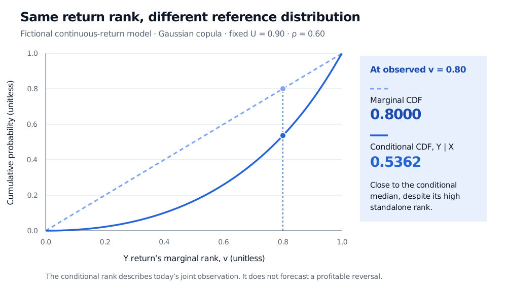
Although

Y

is at its standalone 80th percentile, it is only at about the 53.62nd conditional percentile given

X

’s 90th percentile. Its high marginal rank is largely consistent with the partner’s high rank. Under independence, the conditional rank would instead equal

v=0.80

Fictional Gaussian-copula example with U fixed at 0.90 and rho 0.60. At Y marginal rank 0.80, the conditional CDF is 0.5362, compared with the marginal CDF 0.8000; both axes are unitless.

Original deterministic illustration. The dashed line is the marginal CDF on rank scale; the solid curve is the conditional CDF given $U=0.90$ . This describes the contemporaneous observation, not future performance.

A signal still needs a trading rule

Pairs trading adds a convergence hypothesis and an executable position to that statistical description. A contrarian rule might buy $Y$ and short $X$ when $Y$ is conditionally low and $X$ conditionally high. Those labels describe the fitted distribution, not a no-arbitrage pricing identity. Conditional ranks also supply no unique share hedge ratio or position size.

There are distinct copula strategies. In their 2014 working paper, §§2.2–3.1, Xie, Liew, Wu and Zou fit return marginals and copulas during formation, then accumulate centered daily conditional ranks into trading indicators. An accumulated indicator is a path-dependent score, not itself a probability. Other designs use conditional bounds directly; thresholds, reset conventions, exits and stopping rules therefore belong to the specified strategy. There is no universal “trade above 0.80” rule.

A return copula describes cross-asset dependence at the chosen horizon. It does not by itself establish cointegration of price levels, stationarity of a traded spread, or mean reversion. A better in-sample dependence fit can coexist with worse trading performance.

What an honest backtest must preserve

Three boundaries matter when evaluating this method:

Information availability. Estimate marginals, dependence parameters and pair selection using data available before the signal. Specify rolling refits in advance. A signal requiring the completed closing returns is available after those returns are observed; an assumed fill at that same close needs a feasible execution mechanism. Otherwise use a later executable price. This prevents look-ahead bias.
Distribution stability. Changing volatility can invalidate marginal ranks even if the copula is unchanged; dependence can change independently. Volatility filtering and conditional models are possible choices, not automatic properties of a copula. A Gaussian copula also has zero asymptotic upper and lower tail dependence for $|\rho|<1$ ; it cannot represent every joint-crash pattern. Tail-asymmetric families must be tested against the data, rather than selected because their signals look profitable.
The trade ledger. Fix sizing, borrowing availability, financing, dividends, execution delay and costs for both legs. Compare the complete procedure on held-out dates and account for searching across pairs, copula families and thresholds. In Stander, Marais and Botha’s 2013 study, costs absorbed much of the reported pairs-strategy profit. A statistically unusual observation can be too small, too slow or too expensive to trade.

For the mathematical foundation, SelfMadeQuant’s Copulas and Sklar’s Theorem develops the marginal/dependence separation and probability transforms. The public page is a preview; the full lesson requires membership.

Sources

Xie, W., Liew, R. Q., Wu, Y. and Zou, X. — Pairs Trading with Copulas, 3 May 2014 working paper, §§2.2–3.1.
Haugh, M. — An Introduction to Copulas, 2016, §§1, 2.1 and 3.2.
Frees, E. — Constructing Insurable Risk Portfolios, Appendix §14.1.1.2, Gaussian copula derivatives.
Stander, Y., Marais, D. and Botha, I. — Trading strategies with copulas, 2013, abstract and study scope.

From two returns to two conditional ranks

An 80th percentile that is barely above the conditional median

A signal still needs a trading rule

What an honest backtest must preserve

Sources

Related terms

Cointegration

Cumulative distribution function

Look-ahead bias

Mean reversion

Stationarity