Distinguish Pearson count tests from the normal-variance test, work through synthetic order outcomes, and see why chi-squared p-values need the right calibration.
Chi-squared test
A chi-squared test is a hypothesis test whose statistic is compared with a chi-squared distribution under the null hypothesis. The comparison may be exact under a particular model or only a large-sample approximation. In everyday use, the name usually means Pearson’s test of observed versus expected category counts.
For a quant, that can mean checking whether an execution model predicts the right proportions of fully filled, partly filled and unfilled orders. A large mismatch challenges the model. A small mismatch does not establish that the model is correct, profitable or stable through time.
Choose the question before the formula
Three common uses share a reference distribution, but ask different questions.
Question
Statistic and reference law
What the test addresses
Do category frequencies match specified probabilities?
Pearson’s X2=∑i(Oi−Ei)2/Ei; approximately chi-squared
Goodness of fit
Are two categorical variables independent?
Pearson’s sum across a two-way table; approximately chi-squared with (r−1)(c−1) degrees of freedom
Independence, such as venue versus fill outcome
Does a normal population have a specified variance?
(n−1)S2/σ02; exactly chi-squared with n−1 degrees of freedom for an IID normal sample
A claim about population variance, using the usual sample variance
In the independence case, the expected count in cell (i,j) is the row total times the column total divided by the grand total. Those margins are estimated from the table; the degrees of freedom are not simply the number of cells minus one. Rejection indicates association, without establishing its cause. NIST’s independence-test reference gives this construction and its sampling-design qualifications.
The variance test is a different construction. Here S2 uses denominator n−1, and σ02 is the hypothesised variance. Its exact law requires independent normal observations with a common variance. Heavy-tailed or dependent returns do not inherit that guarantee. Depending on the alternative, unusually low variance, unusually high variance or both can lead to rejection; an upper-tail Pearson recipe cannot be copied indiscriminately. See NIST’s variance-test reference.
An execution model under scrutiny
Consider 100 synthetic orders, treated as independent and identically distributed categorical observations. Before seeing their outcomes, the model specifies probabilities 0.4, 0.4 and 0.2 for fully filled, partly filled and unfilled orders, respectively. Each order receives exactly one final classification at a fixed assessment time; the categories are disjoint and exhaustive.
The null hypothesis fixes all three probabilities. No parameter is estimated from these 100 outcomes. Under that null, the count vector has a multinomial distribution. For category i, its expected count is Ei=npi,0, where pi,0 is its null probability.
Final order outcome
Null probability
Observed Oi
Expected Ei
Contribution (Oi−Ei)2/Ei
Fully filled
0.4
50
40
2.5
Partly filled
0.4
30
40
2.5
Unfilled
0.2
20
20
0
Total
1
100
100
5
Squaring prevents the excess of fully filled orders from cancelling the shortfall of partly filled orders. Dividing by the expected count scales each discrepancy: the same absolute count error has a larger contribution in a rarer category. The statistic loses the direction of each discrepancy, so keep the observed-minus-expected signs alongside it.
There are three counts but their total is fixed. Once two counts are known, the third is determined. With no fitted null parameters, the reference has 3−1=2 degrees of freedom:
X2=40(50−40)2+40(30−40)2+20(20−20)2=5.
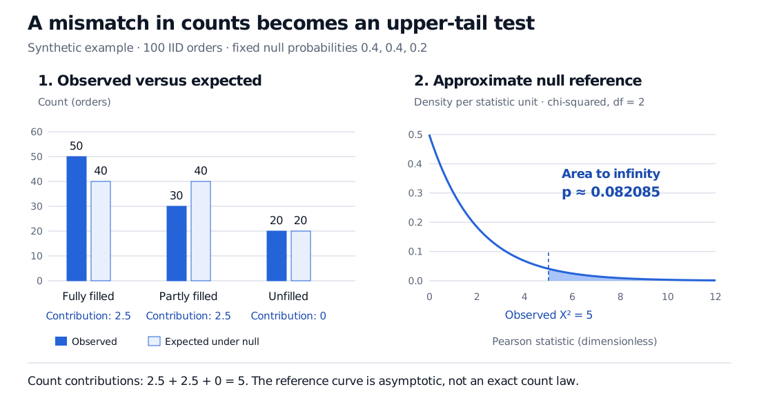
Synthetic order counts: observed 50, 30 and 20 versus expected 40, 40 and 20. Pearson contributions are 2.5, 2.5 and 0, giving X squared 5. The chi-squared reference with two degrees of freedom gives upper-tail p approximately 0.082085.
Original synthetic example. Left: order counts and contributions. Right: the continuous, asymptotic reference density; the shaded probability extends beyond the displayed axis to infinity.
For two degrees of freedom, the chi-squared survival function has a particularly simple form. The approximate p-value is
pasym=P(χ22≥5)=e−5/2≈0.082085.
At a prespecified significance level of 5%, this does not reject the null. The upper 5% critical value is about 5.991, above the observed statistic of 5. The p-value is not an 8.2% probability that the execution model is true. It measures an upper-tail discrepancy probability under the null reference, conditional on the stated design.
Integer counts do not make the chi-squared approximation exact. In this small, fully specified example, one can enumerate every possible count triple summing to 100. Summing its multinomial probability whenever its Pearson statistic is at least 5 gives an exact finite-sample tail probability of about 0.088928. That differs from 0.082085 because the actual statistic has a discrete distribution, while the chi-squared reference is continuous. Both give the same decision at 5%; they are different calibrations of the same discrepancy statistic.
What must survive contact with real data
Inspect expected counts, not just the sample size. A large total can conceal near-empty expected categories. All expected counts here are at least 20, supporting the usual approximation, though no threshold alone proves accuracy. “Expected counts at least five” is a common screening rule, not an exactness theorem. Sparse designs may need an exact multinomial calculation or a suitable null simulation; contingency tables have their own exact-test options. NIST’s goodness-of-fit discussion explains the role of binning and fitted parameters.
The observations must have the claimed sampling structure. The category counts themselves are dependent because they sum to 100; that dependence is already built into the multinomial model. The important assumption is independence across the underlying orders. Orders from the same parent trade, clustered market conditions or repeated measurements of one order can violate it. Pooling such observations and increasing the nominal sample size does not repair the test.
Estimating the null changes the calibration. For a regular multinomial model with k fixed categories and q identifiable null parameters fitted by maximum likelihood to the grouped counts, the usual asymptotic degrees of freedom are k−1−q. This is not permission to subtract any number of parameters from any workflow. Fitting a continuous distribution to raw observations and then binning them can change the limiting law; boundary constraints and data-selected bins also need care. Simulation-based calibration must reproduce the fitting and selection steps being assessed.
Read the discrepancy economically. Here fully filled orders exceed expectation by ten while partly filled orders fall short by ten. That identifies where to investigate classification, order mix or model assumptions. It does not tell us whether transaction costs improved, and failure to reject cannot certify future execution quality. Repeating the test across many venues or windows also introduces multiple testing.
For the derivation and a deeper treatment of fitted probabilities, read Goodness-of-Fit Tests. The public page offers a preview; the full lesson requires membership. Its discussion of grouped versus ungrouped estimation is especially useful before adapting a count test to continuous financial data.
Sources
John A. Rice, Mathematical Statistics and Data Analysis, third edition, §9.5, “Likelihood Ratio Tests for the Multinomial Distribution”; §9.9, “Tests for Normality” (grouped-estimation caveat); §6.3, “The Sample Mean and the Sample Variance.”